QGIS#
A QGIS-based workflow to support the computation of SDG Indicator 15.4.2, which includes: sub-indicator a (Mountain Green Cover Index) and sub-indicator b (Proportion of degraded mountain land).
General Information#
About QGIS-SDG 15.4.2 beta#
This documentation and geospatial workflow has been developed by the UN Environment Programme World Conservation Monitoring Centre (UNEP-WCMC) in collaboration with the Food and Agriculture Organization (FAO) of the United Nations to support relevant national authorities to compute and report against SDG Indicator 15.4.2.
The geospatial workflow was developed using QGIS 3.28.11, a free and open-source geographic information system licensed under the GNU General Public License. QGIS is an official project of the Open Source Geospatial Foundation (OSGeo). It runs on Linux, Unix, Mac OSX, Windows and Android and supports numerous vector, raster, and database formats and functionalities. To run this workflow, you will also need to have R Software installed.
The QGIS-SDG 15.4.2 beta workflow is in a beta stage and therefore it is still under development. Please contact the QGIS-SDG 15.4.2 beta development team with any comments or suggestions.
If you have specific bugs to report or improvements to the tool that you would like to suggest, please use the GitHub’s issue tracker of the QGIS-SDG 15.4.2 beta module and do follow the contribution guidelines.
Suggested Citation#
UNEP-WCMC and FAO (2023) SDG 15.4.2 Computation: Technical documentation for QGIS to aid the calculation of SDG Indicator 15.4.2: (a) Mountain Green Cover Index and (b) proportion of degraded mountain land. United Nations Environment Programme World Conservation Monitoring Centre, Cambridge.
License#
The QGIS-SDG 15.4.2 beta workflow and its documentation is made available under the terms of the Creative Commons Attribution 4.0 International License (CC BY 4.0) .
Initial setup#
QGIS software installation#
Ensure QGIS 3.22.16 installed on your computer. We suggest users use the Long-Term Release version of QGIS to undertake their analysis as this is the most stable version and users are less likely to incur technical difficulties and bugs. There are various installers depending on your operating system but for most users we recommend the QGIS Standalone Installer. Full instructions are on their website: https://qgis.org/en/site/forusers/download.html.
While the QGIS-SDG 15.4.2 beta analysis runs entirely within the QGIS interface, to run this workflow, you will also need to install R Software 4.4.1. R scripts will be run from within the QGIS interface and no prior knowledge of R is required. There have been a number of releases since 4.4.1 we have found that some of the later versions cause the r-scripts to run slower within the toolbox.
R software and packages installation#
Download and install R from https://www.r-project.org/ and then download and install RStudio Desktop from https://www.rstudio.com/products/rstudio/. A step-by-step guide on how to install R and R Studio (with images) can be found in Annex 1.
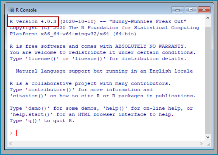
It is important to use a current version of R software (we currently recommend R-4.1.3). Although there have been a number of releases since 4.1.3, we have found that some of the later versions cause the r-scripts to run considerably slower within the QGIS toolbox. If you already have R installed, the R version can be easily checked on the text within the ‘R Console’ box at the beginning of a new session (see Figures below for standalone R and R Studio). You can have multiple versions of R installed on your computer at a time so if you don’t have this version.

QGIS-SDG 15.4.2 custom toolbox download and extraction#
Users will also need to download the SDG_15_4_2_beta_Toolbox and set of templates and style files from the SDG_15_4_2_beta repository. In a web browser navigate to the SDG15.4.2 beta repository using the following URL: https://github.com/sepal-contrib/wcmc-mgci/tree/main
Click on Code>>Download ZIP
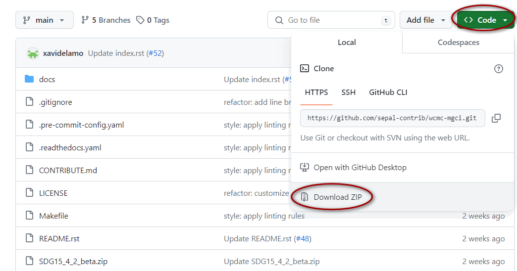
Next open a file explorer window and navigate to the folder where you have downloaded the file. At this stage we would recommend you move the zip file to a sensible location with a short and simple file structure. e.g. in this example we have moved the downloaded zip file to c:\workspace. Right-click on the file named wcmc-mgci-main.zip and click on 7-ZIP >>Extract here.

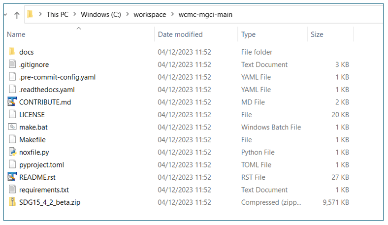
Once unzipped you should see a folder of the same name (wcmc-mgci-main). Navigate inside this folder and you should see the following file structure and a zip file called SDG15_4_2_beta.zip.
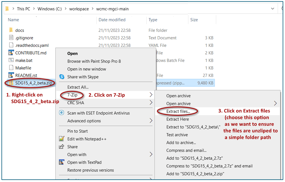
Right-click on SDG15_4_2_beta.zip and click on 7-ZIP>>Extract file. Note we are clicking on extract files this time and not extract here as we want to make some modifications to the path we are unzipping to.
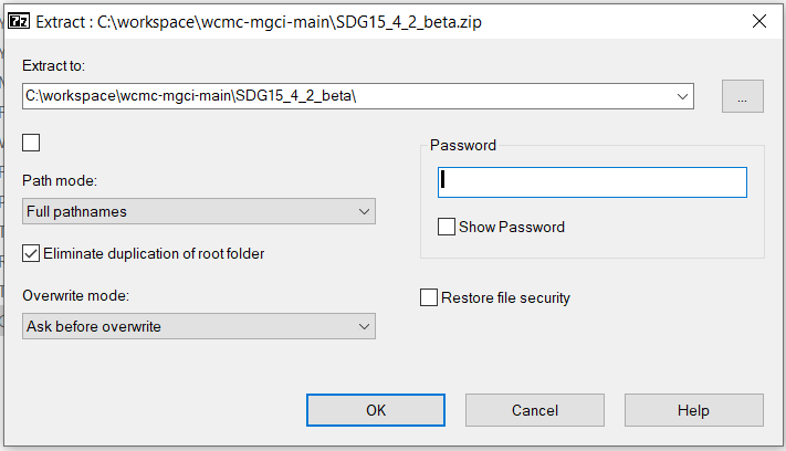
You should see the unzip files window below. Do NOT click OK yet as we want to make some changes.
First remove ‘wcmc-mgci-docs-main’ from the extract to path and then tick Eliminate duplication of root folder.
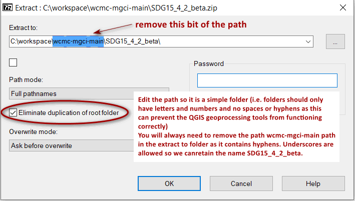
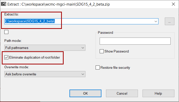
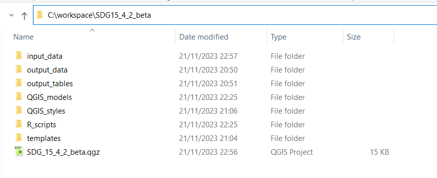
Click okay once you have done these steps. You should now have a folder set up for the QGIS processing. Please do not alter the folder structure as the tools rely on these to remain intact.
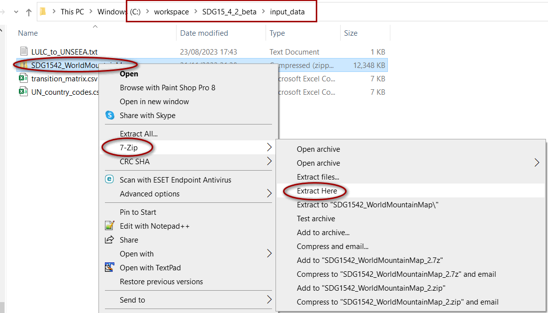
The next step is to go into the input_data folder and unzip the Global mountains map. Right-click on SDG1542_WorldMountainMap.zi and click on 7-ZIP>>Extract here.
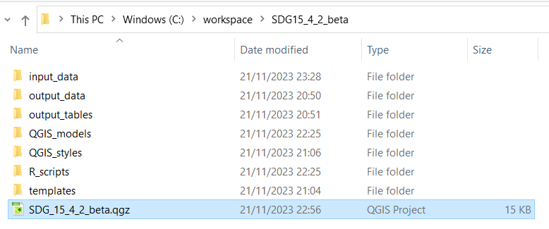
You are now ready to open the QGIS project. Double-click to SDG_15_4_2_beta.qgz to open the project.
QGIS-SDG 15.4.2 custom toolbox and plugins installation#
Next (once QGIS is open) there are a few steps that need to be undertaken to set up the QGIS project correctly and to link it to the custom toolbox and scripts.
First you will need to install the following plugins:
Processing R Provider: This plugin essentially allows R scripts to be used directly within the QGIS processing toolbox with the simple addition of some QGIS header information placed at the top of the script to making the R script behave exactly like other processing tools in the QGIS processing toolbox. The header information allows graphical fields to be set in the processing dialogue window when running the tool e.g. the input raster, a specific field or the location and name of an output raster. Some header information is used to tell QGIS to either pass information to R and from QGIS about the tool to enable the R processing to happen within the QGIS interface.
From the QGIS Menu Toolbar click on Plugins>>Manage and Install Plugins

From the Plugin dialogue window search for processing R
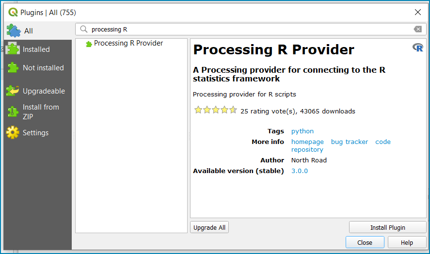
Click Install Plugin and then Close
The Processing R Provider has now been installed.
Updating QGIS settings#
Next some QGIS settings will be changed to ensure QGIS knows where to find the R installation, scripts and model folders.
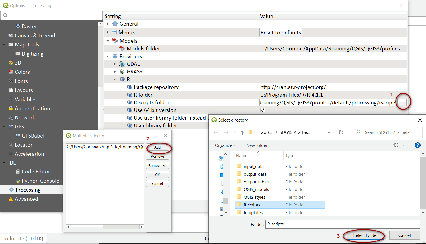
From the main menu select settings>>processing. Click on providers and expand the R tab. Double click on the R-scripts folder path to expose the three dots. Click on this and click Add. Navigate to the R_scripts folder in the SDG15_4_2_beta folder. e.g. in this example C:\workspace\SDG15_4_2_beta\R_scripts. Then click OK.
Double-click on the R folder path and navigate to where you have installed your R software. This is to tell QGIS where to run R from. i.e. to check the R folder is pointing to the correct location (where it is installed on your computer)
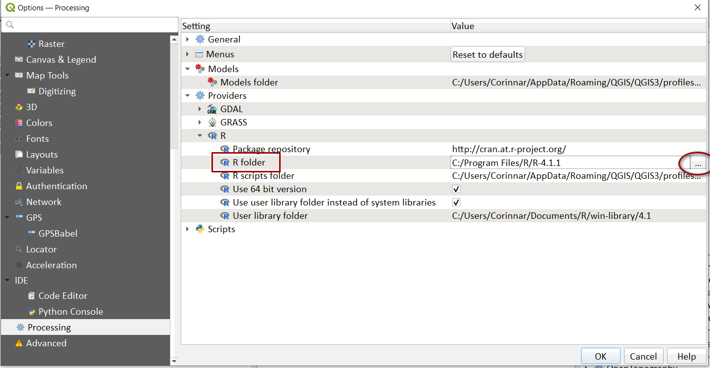
If you operating system is 64 bit, tick Use 64bit version
Click OK
In the same settings>>processing window, shrink down the R tab and expand Model. Double click on the models path to expose the three dots. Click on this and click Add.
Navigate to the QGIS models folder in the SDG15_4_2_beta folder. e.g. in this example C:\workspace\SDG15_4_2_beta\QGIS_models. Then click OK.
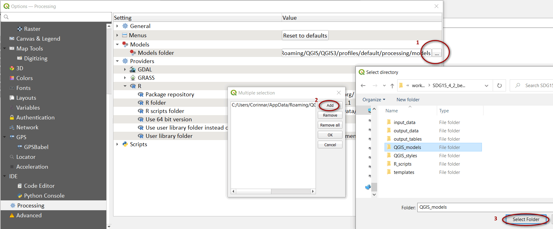
In the same settings>>processing window, shrink down the Model tab and expand Scripts. Double click on the models path to expose the three dots. Click on this and click Add.
Navigate to the QGIS scripts folder in the SDG15_4_2_beta folder. e.g. in this example C:\workspace\SDG15_4_2_beta\QGIS_scripts. Then click OK.

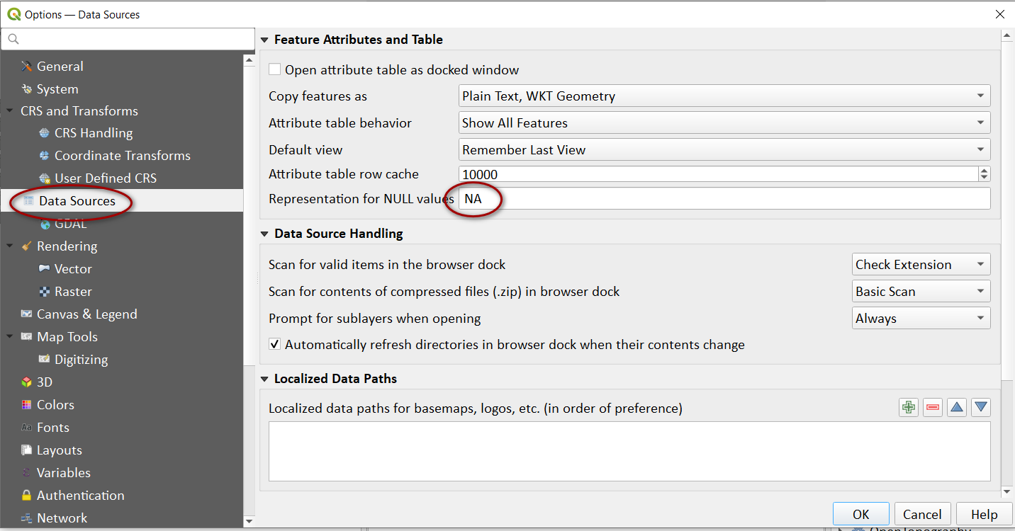
Next on the left hand panel click on Data Sources and change the Representation of null values from Null to NA (this will ensure the correct NA representation of Null values in the output reporting tables).
In the same settings window click on processing>>general and change the Results group name to OUTPUTS. Put this in capitals as this is how it will then appear in the QGIS table of contents. It means that any outputs from geoprocessing tools will be stored under this group heading and makes it easier to distinguish from the INPUT data.
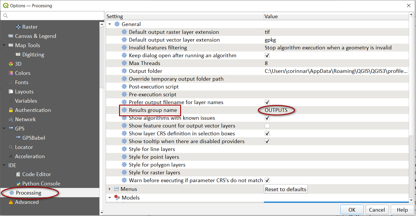
Once done click OK to close the setting window and return to the main QGIS interface.
On the right-hand side of QGIS you should see the processing Toolbox. (If it is not visible, from the main menu select View>>panels>>processing toolbox).
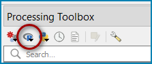
You should also see that the R script button has appeared on the processing toolbox menu and R scripts tab visible in the toolbox.
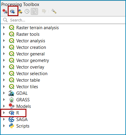
In the processing toolbox if you expand models and R you should see the SDG15.4.2 models and scripts present. It is from the toolbox that you will run the tools if you choose to use the SDG_15_4_2_beta toolbox rather than undertaking the manual steps.
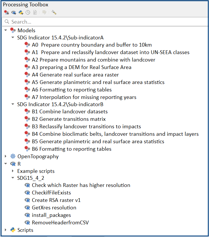
Save the QGIS project.
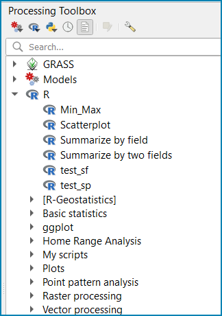
Optional step: Add the Resource sharing plugin: This plugin is a useful R related plugin (which is not essential for the MGCI but useful for users wishing to integrate R with QGIS).
Once the resource sharing plugin is installed some additional scripts will also be visible. They are grouped into several categories as in the screengrab below.
To add this plugin click on plugins>>resource sharing>>resource sharing
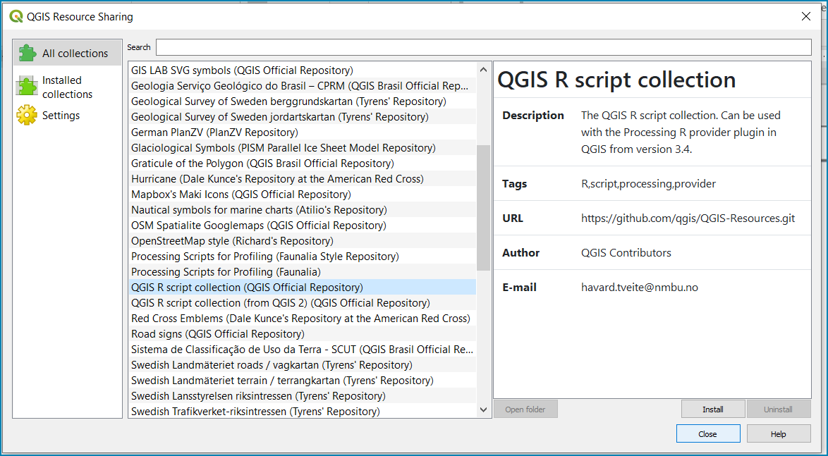
Click on All Collections on the left hand panel and click QGIS R script collection (QGIS Official Repository) then click Install
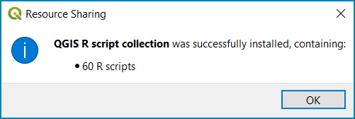
The wider collection of scripts should now be present in the R-scripts collection. These are not required for MGCI but useful for R-Integration with QGIS.
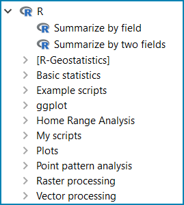
For further information see the following sections of the QGIS user manual at
https://docs.qgis.org/3.28/en/docs/user_manual/processing/3rdParty.html#r-libraries
Running analysis steps using the custom QGIS toolbox#
This section of the tutorial explains in detail how to calculate value estimates for sub-indicator 15.4.2a in QGIS, using Colombia as a case study. This section assumes that the user has already downloaded the global mountain map made available by FAO to compute this indicator and a land cover dataset meeting the requirements described in the Background section.
We provide the SDG_15_4_2_beta toolbox custom toolbox to group and run the steps to help speed up the analysis and allow for easier repeat processing and to standardize the naming of outputs and how they appear within the QGIS interface.
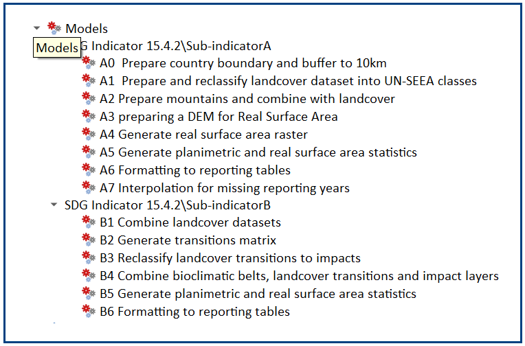
For each step we provide a tool diagram to illustrate the steps being undertaken within the toolstep, however Annex 2 of the tutorial outlines in detail the main steps each tool undertakes in the SDG 15.4.2 processing toolbox. This can be used as a reference if the user wishes to understand how each tool step would be carried out manually. Note that some plugins such as GroupStats and OpenDEMDownloader (which have been explained in steps in Annex 2) are not supported easy to implement on model builder in QGIS. Therefore, it was more efficient to use slightly different approaches for the model builder in such cases.
Instructions to calculate Sub-indicator 15.4.2a in QGIS using the custom models#
This section of the tutorial explains in detail how to use the custom QGIS toolbox to calculate value estimates for sub-indicator 15.4.2a in QGIS, using Colombia as a case study.
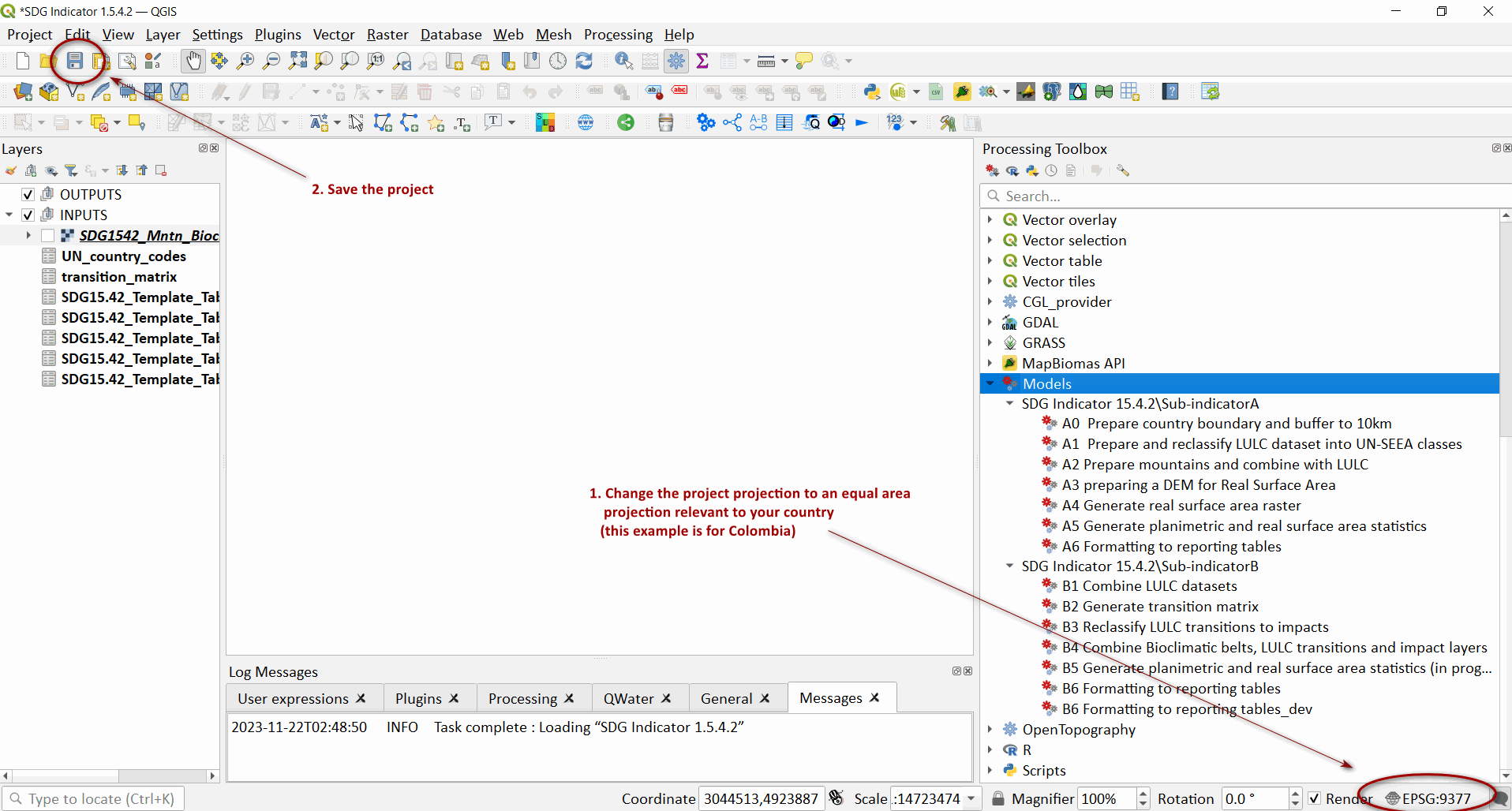
Before we begin running the tools at this stage we want to set-up the projection for the analysis. We therefore want to set the project window to an equal area projection. For choosing an equal are projection for your country please see the Defining projections to be used for the analysis section for guidance).
Click on the project projection EPSG: 4326 in the bottom right hand corner of the QGIS project

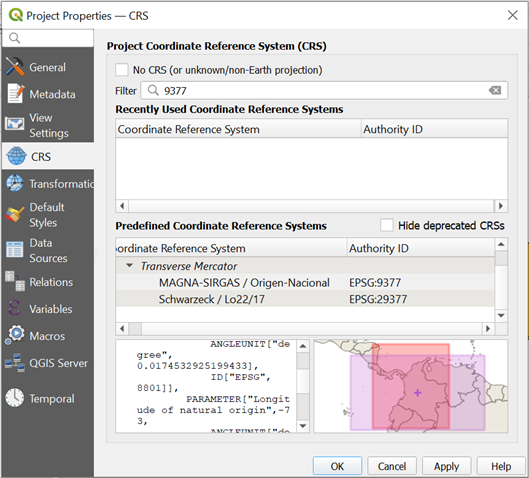
In the Project Properties dialogue window search for the chosen projection in the Filter tab, in this case the projection EPSG 9377
Step A0 Prepare country boundary and buffer to 10 km#
The first step is to define the Area of Interest (AOI) for the analysis. This should go beyond the country boundary as outlined in the Defining an area of interest section of the tutorial. In this example, the input boundary layer is in Geographic coordinate system (EPSG 4326). At this stage we want to set-up the projection for the main parts of the analysis. We therefore want to set the project window to an equal area projection and physically project the country boundary to the same projection.
Colombia does have a National Projection that preserve both area and distance (see here) and therefore could be used as a custom projection. In case a national projection that minimize area distortion does not exist for a given country, it is recommended to define a custom Equal Area projection centered on the country area following the instructions in described here under Defining projections to be used for the analysis section).
In the Processing Toolbox, under Models, click on model A0 Prepare country boundary and buffer to 10 km
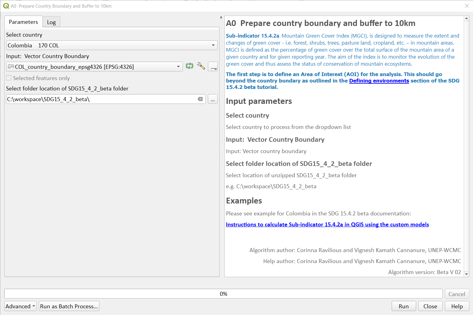
Input parameters
Follow the instructions in the right-hand panel of the tool interface (see screengrab above)
Click Run
This will generate the country boundary in equal area projection and one with a 10 km buffer around the country boundary.
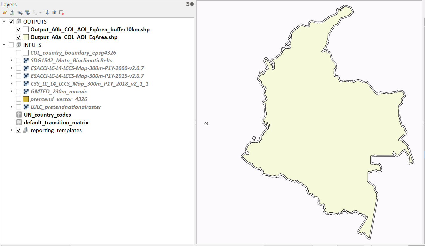
The boundaries and names shown, and the designations used on this map do not imply official endorsement or acceptance by the United Nations.
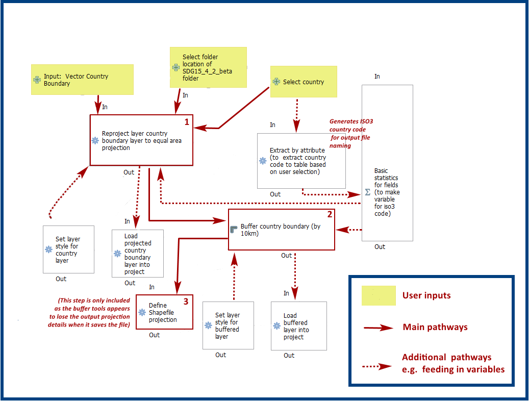
Tool A0 model diagram
Now that the country boundary is in the chosen projection, we can generate the land cover and mountain maps for Colombia.
Step A1 Prepare and Reclassify LULC Dataset into UN-SEEA Classes#
The next step is to reclassify your chosen land cover dataset into the UN-SEEA classification. Preferably a National landcover raster dataset should be used. To demonstrate the steps for processing a raster land cover dataset we will use the Global ESA CCI landcover dataset.
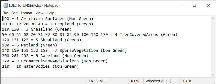
If the land cover dataset is a regional or global extent it will need projecting and clipping to the AOI. In this example we are using a global dataset so we will need to clip the raster and save it in the equal area projection. Next, we reclassify the land cover map into the 10 UN-SEEA classes defined for SDG Indicator 15.4.2. QGIS provides several tools for reclassification. The easiest one to use in this instance is the r.reclass tool in the GRASS toolset as it allows the upload of a simple crosswalk text file containing the input LULC types on the left and the UN-SEEA reclass values on the right. Create a text file to crosswalk land cover types from the ESA CCI or National land cover dataset to the 10 UN-SEEA land cover classes.
First we will run for the year 2000.
In the Processing Toolbox, under Models, click on model A1 Prepare and reclassify land cover dataset into UN-SEEA classes.
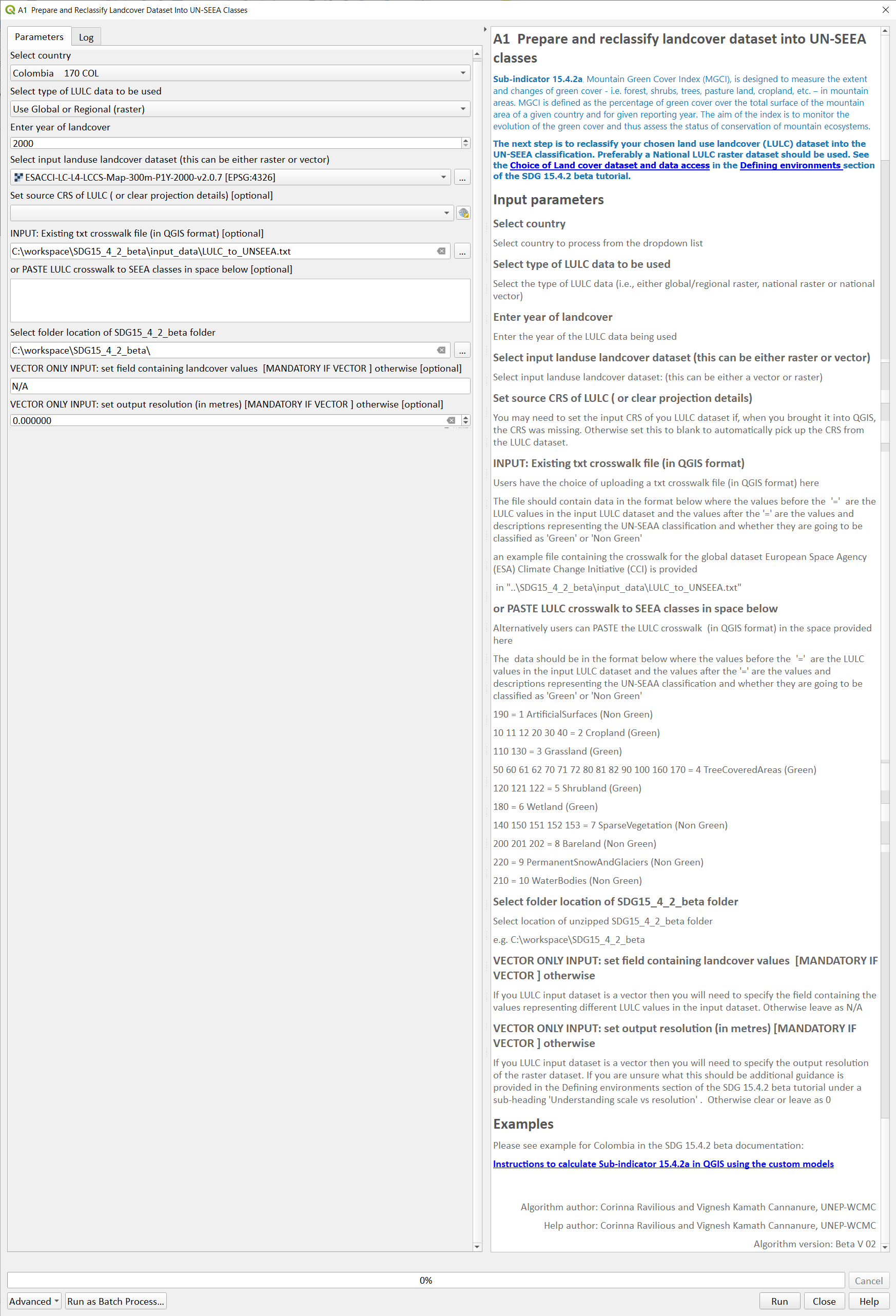
Input parameters
Follow the instructions in the right-hand panel of the tool interface (see screengrab above)
Click Run.
You should now see the unique land cover classes present within the AOI for the country.
You can run subsequent years by then clicking Change parameters and change the LULC to e.g. the 2015 dataset and year to 2015. Click Run. Repeat this until you have run all the years you wish to run.
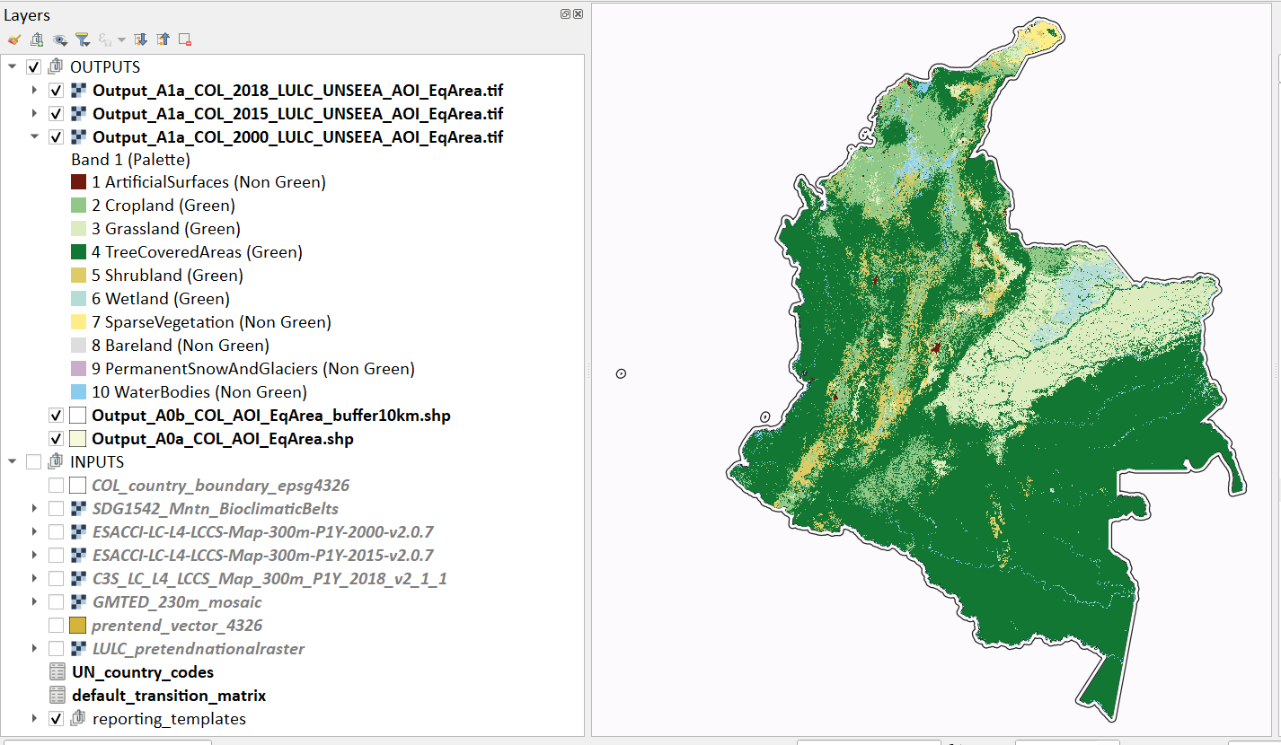
The boundaries and names shown, and the designations used on this map do not imply official endorsement or acceptance by the United Nations.
Tool A1 model diagram

Step A2 Prepare mountain layer and combine with LULC#
The development of mountain map consists in clipping and reprojecting the SDG 15.4.2. Global Mountain Descriptor Map developed by FAO to area of interest, in this case, the national border of Colombia. Once we have the two raster datasets in their native resolutions, we need to bring the datasets together and ensure that correct aggregation is undertaken and that the all the layers align to a common resolution. As SGD Indicator 15.4.2a requires disaggregation by both the 10 land cover classes and the 4 bioclimatic belts and the tools within QGIS will only allow a single input for zones, we will combine the two datasets. We need to ensure that the layers are aggregated to a common spatial resolution. During this step we ensure we maintain the resolution of the Lamdcover dataset as this is the most import layer in the analysis, rather than the mountain layer as this is only used to determine mountain extent and report on the disagregated values.
First we will run for the year 2000.
In the Processing Toolbox, under Models, click on model A2 Prepare mountains and combine with land cover.
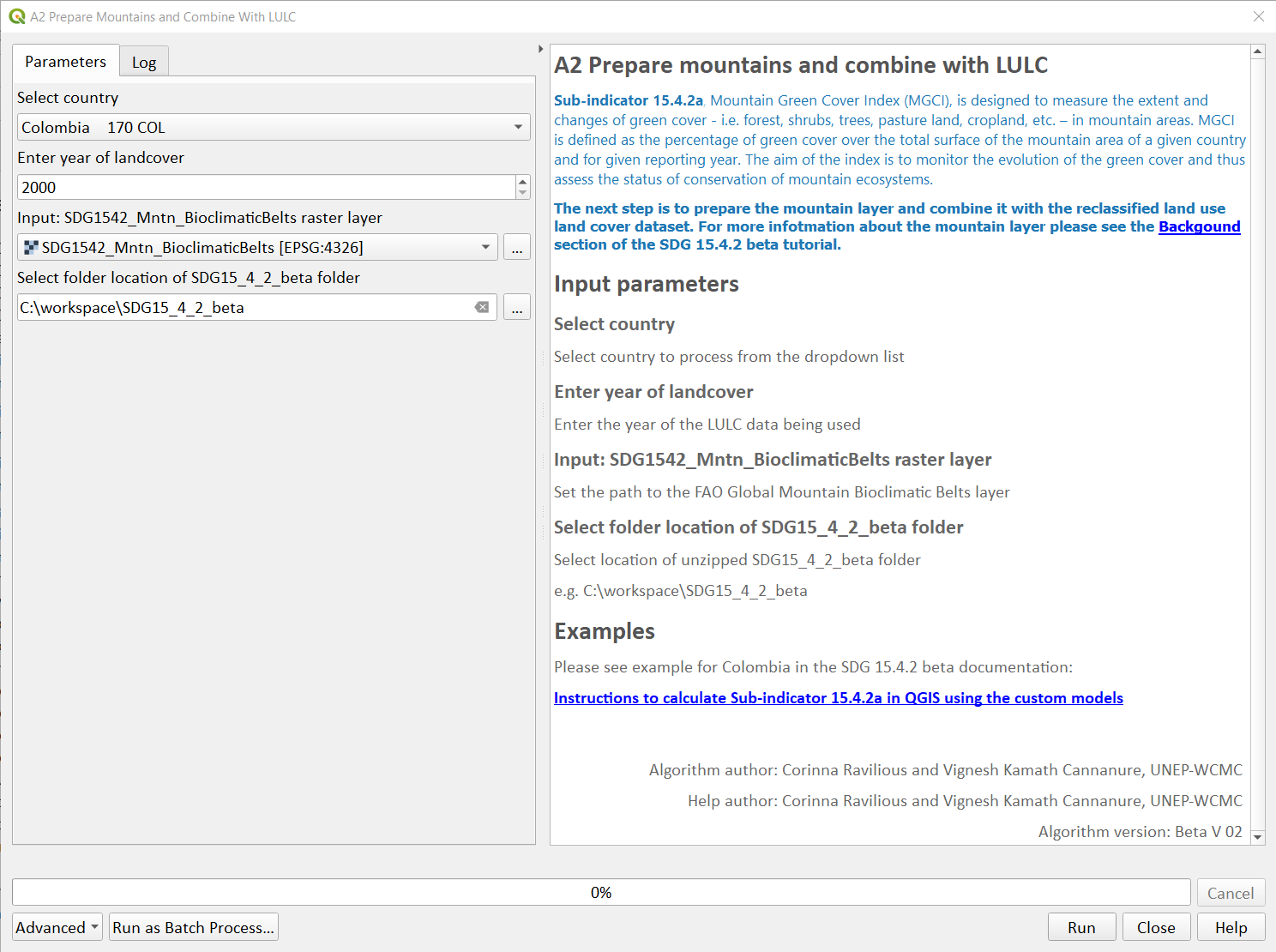
Input parameters:
Follow the instructions in the right-hand panel of the tool interface (see screengrab above)
Click Run.
You can run subsequent years by then clicking Change parameters and change the landcover to e.g. the 2015 dataset and year to 2015. Click Run. Repeat this until you have run all the years you wish to run.
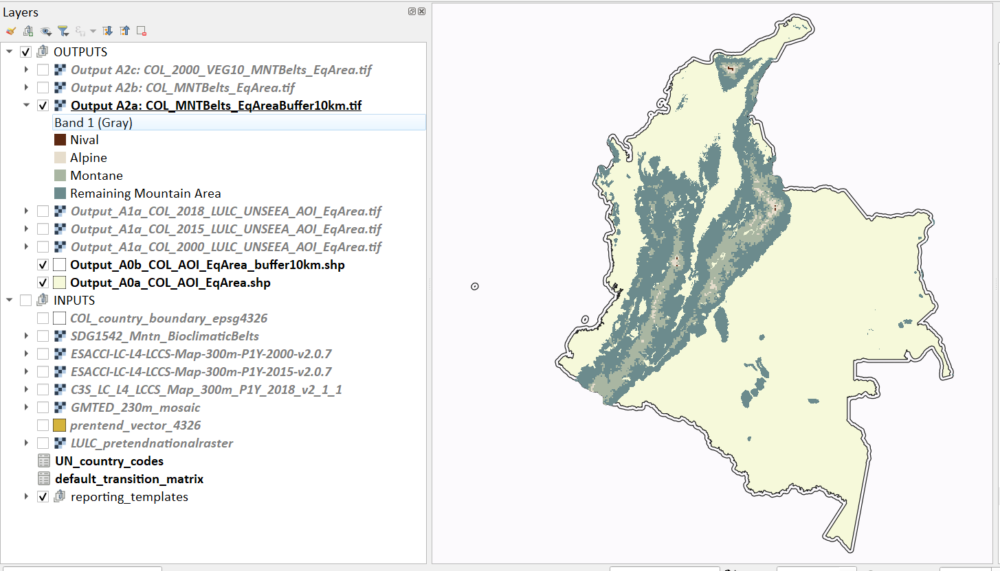
This should produce the following outputs on the map canvas:
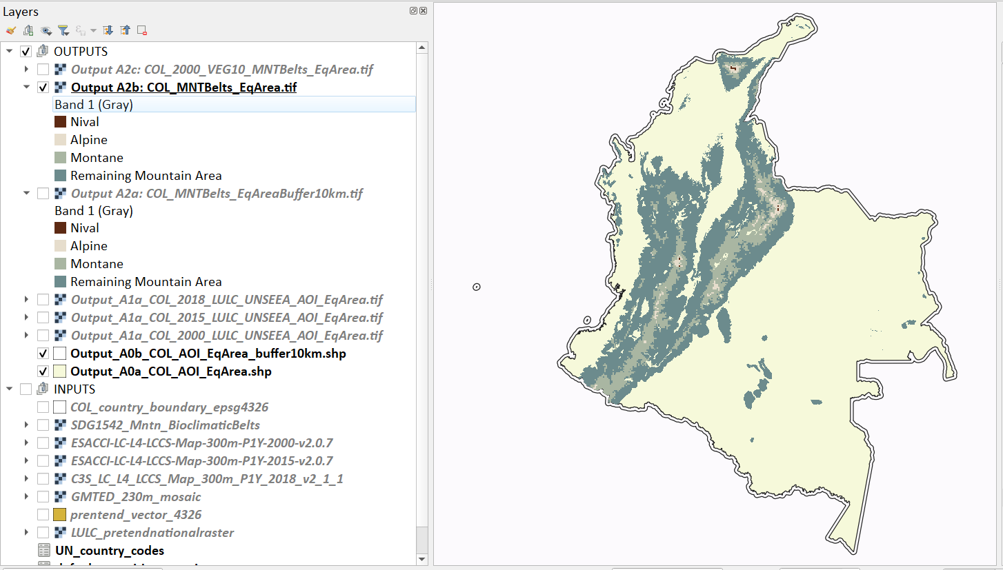
The new clipped mountain descriptor dataset in the national projection. The layer should now show all the mountain area for Colombia classified by Bioclimatic belts (where 1 is ‘’Nival”, 2 is “Alpine”, 3 is ‘’Montane” and 4 is “Remaining Mountain Area”.
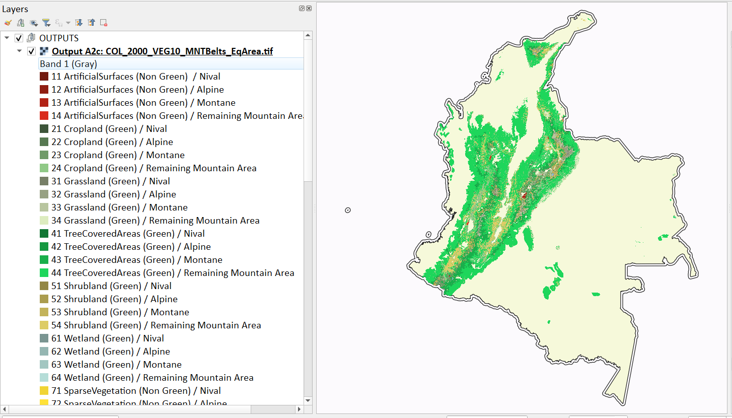
The combined mountain and vegetation layer. In order to distinguish the vegetation class from the mountain all the vegetation values will be multiplied by 10. This means for example a value of 35 in the output means the pixel has class 3 in landcover layer and class 5 in the Mountain descriptor layer.
Result A2a is the global mountain map in its native resolution clipped to the country buffer to reduce the loss of data around the edges when clipping to the country boundary at the landcover resolution:
Result A2b is the global mountain map in its landcover resolution clipped to the country boundary:
Result A2c is the combined landcover and mountain map in its landcover resolution clipped to the country boundary:
The boundaries and names shown, and the designations used on this map do not imply official endorsement or acceptance by the United Nations.
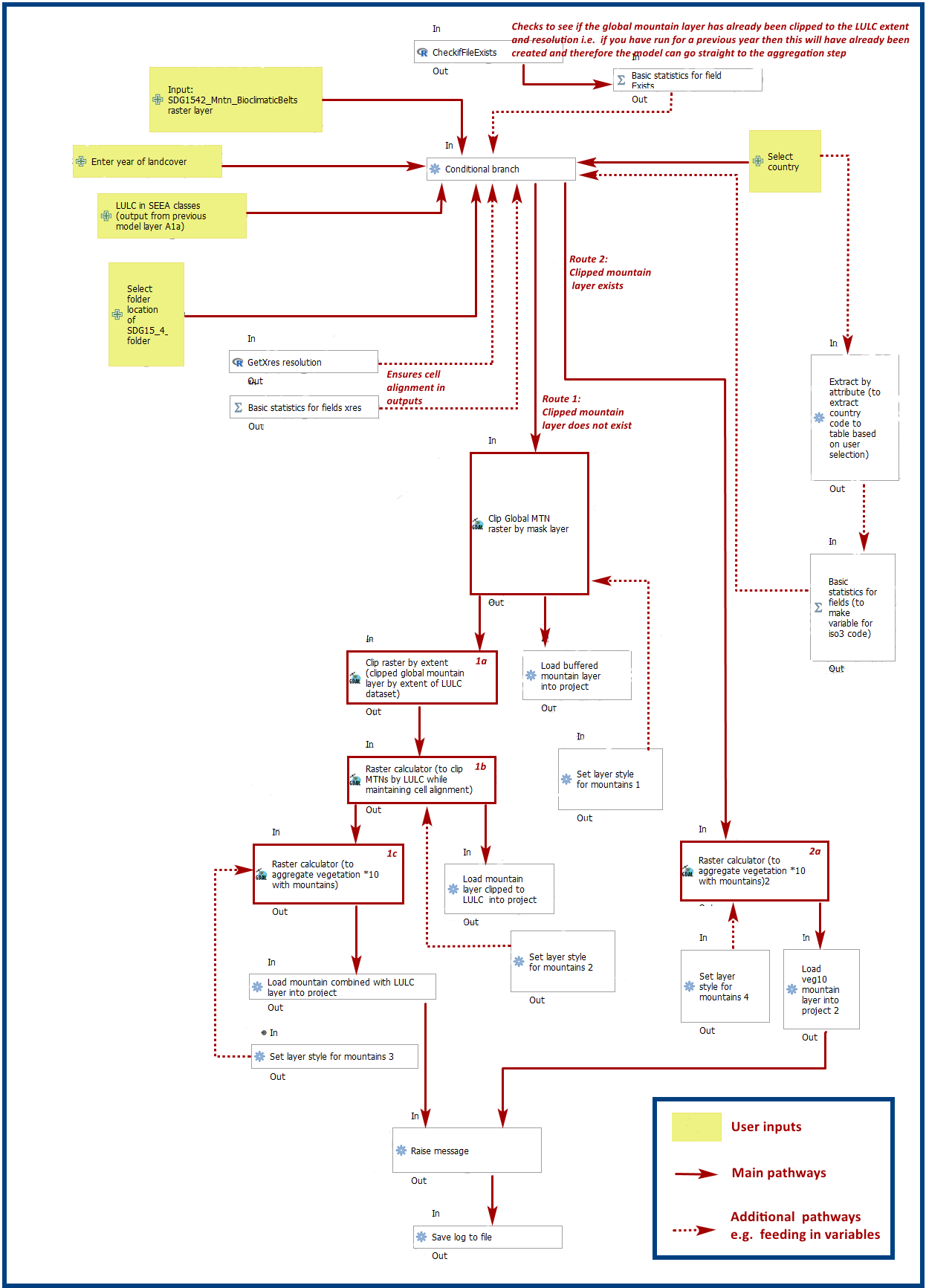
Tool A2 model diagram
Step A3 preparing a DEM for Real Surface Area#
This Step does not run a tool but provides users with information to guide them to the relevant sections in the resources.
For reporting on SDG 15.4.2 countries must report planimetric area. Countries also however have the option to also calculate real surface area. This requires development of a real surface area layer requires a Digital Elevation Model (DEM).
If you are choosing NOT to calculate real surface area, then you can go straight to step A4 as the DEM is only required for this calculation,
Otherwise: If you are choosing to calculate Real Surface Area and you already have a country DEM, you need to ensure that it goes at least 7km beyond the country boundary in all directions as the and is at a resolution that is the same or higher resolution than your landcover dataset then: Load your DEM into the QGIS project
(Note: The higher the resolution (smaller the grid cells), the more detailed information. Higher resolution DEMs can improve the accuracy of analysis however, they are more computationally expensive to use, particularly over large extents.)
The selection of which DEM to use for this can be chosen by the countries. We do not advise countries which DEM to choose although table in section Choice of DEM for generating real surface area calculations and data access in the Defining environments section provides some suggestions for open access sources. There are also some step-by-step guidance in Annex 1 to help use some of the different download options.
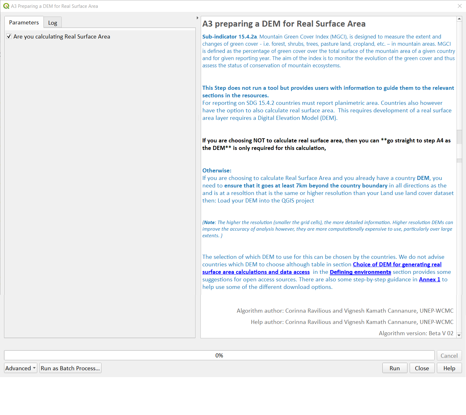
These instructions are also present in the right-hand panel of the tool interface Step A3. The tool step A3 does not actually run anything other than pointing users to the documentation.
Step A4 Generate real surface area raster#
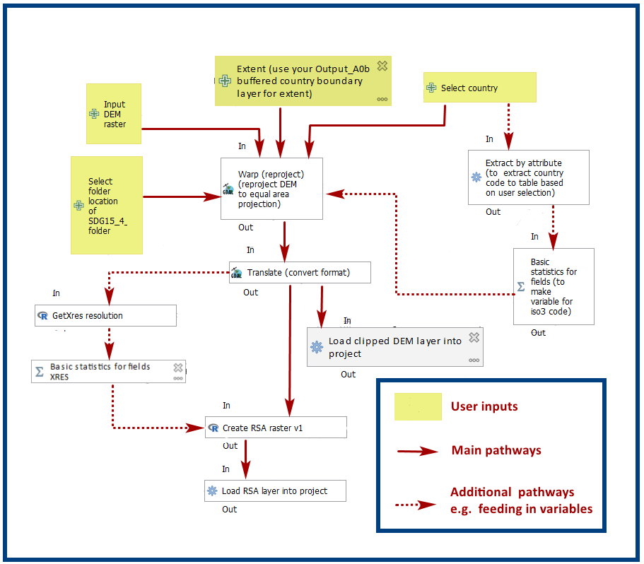
The final layer that needs generating is the Real Surface Area raster from the DEM. The tools should have all been tested to check your R integration is working in the initial setup. Refer to the workflow diagram in the overview section for an explanation of the process to calculate the real surface area from a DEM.
For the purposes of this example we will use a global DEM at 230m resolution as the landcover dataset that we are using in this example is 300m resolution so the DEM has a higher the resolution (smaller the grid cells).
In the Processing Toolbox, under Models, click on model A4 Generate Real Surface Area Raster.
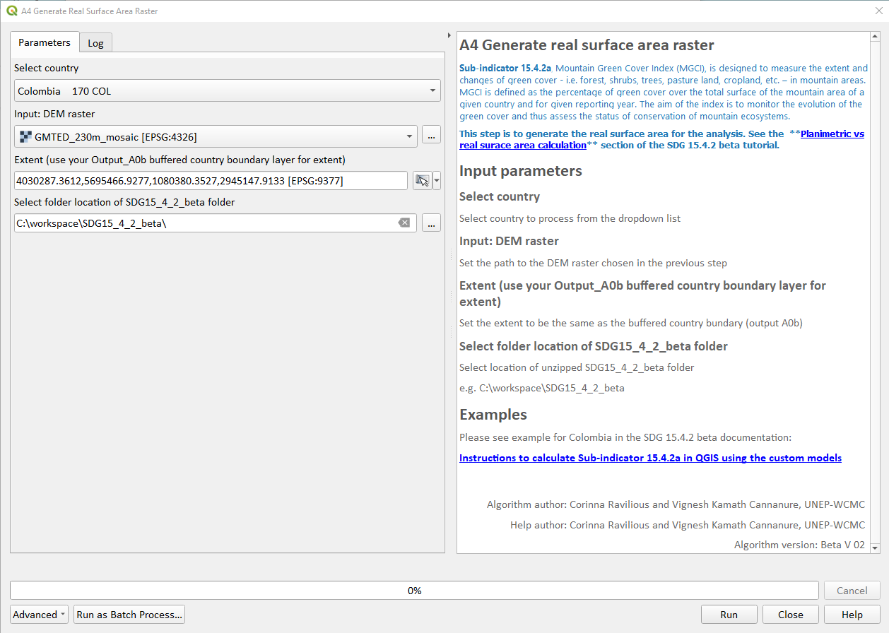
Input parameters:
Follow the instructions in the right-hand panel of the tool interface (see screengrab above)
Click Run.
This should produce the following outputs (a DEM raster and Real Surface Area raster) on the map canvas:
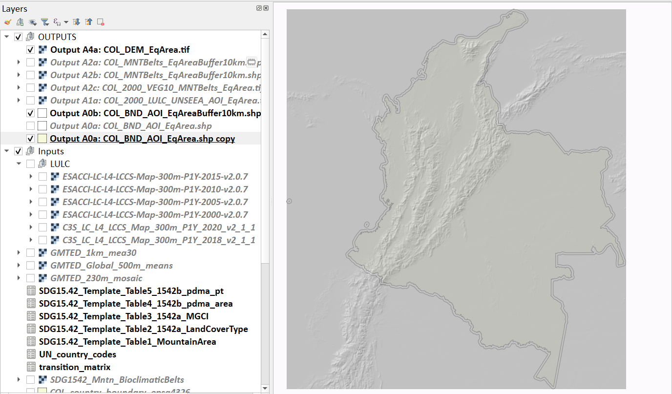
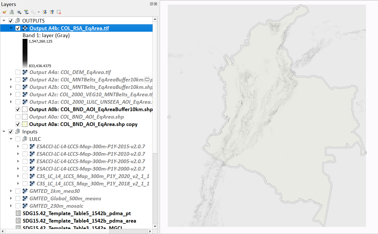
The boundaries and names shown, and the designations used on this map do not imply official endorsement or acceptance by the United Nations.
Tool A4 model diagram
Step A5 Generate planimetric and real surface area statistics#
The data are now in a consistent format, so we can now generate the statistics required for the MGCI reporting. As we want to generate disaggregated statistics by landcover class and bioclimatic belt we will use a zonal statistics tool with the combined landcover + mountain layer as the summary unit. The Zonal statistics tool will automatically calculate planimetric area and real surface area in the output.
In the Processing Toolbox, under Models, click on model A5 Generate Planimetric and Real Surface Area Statistics.
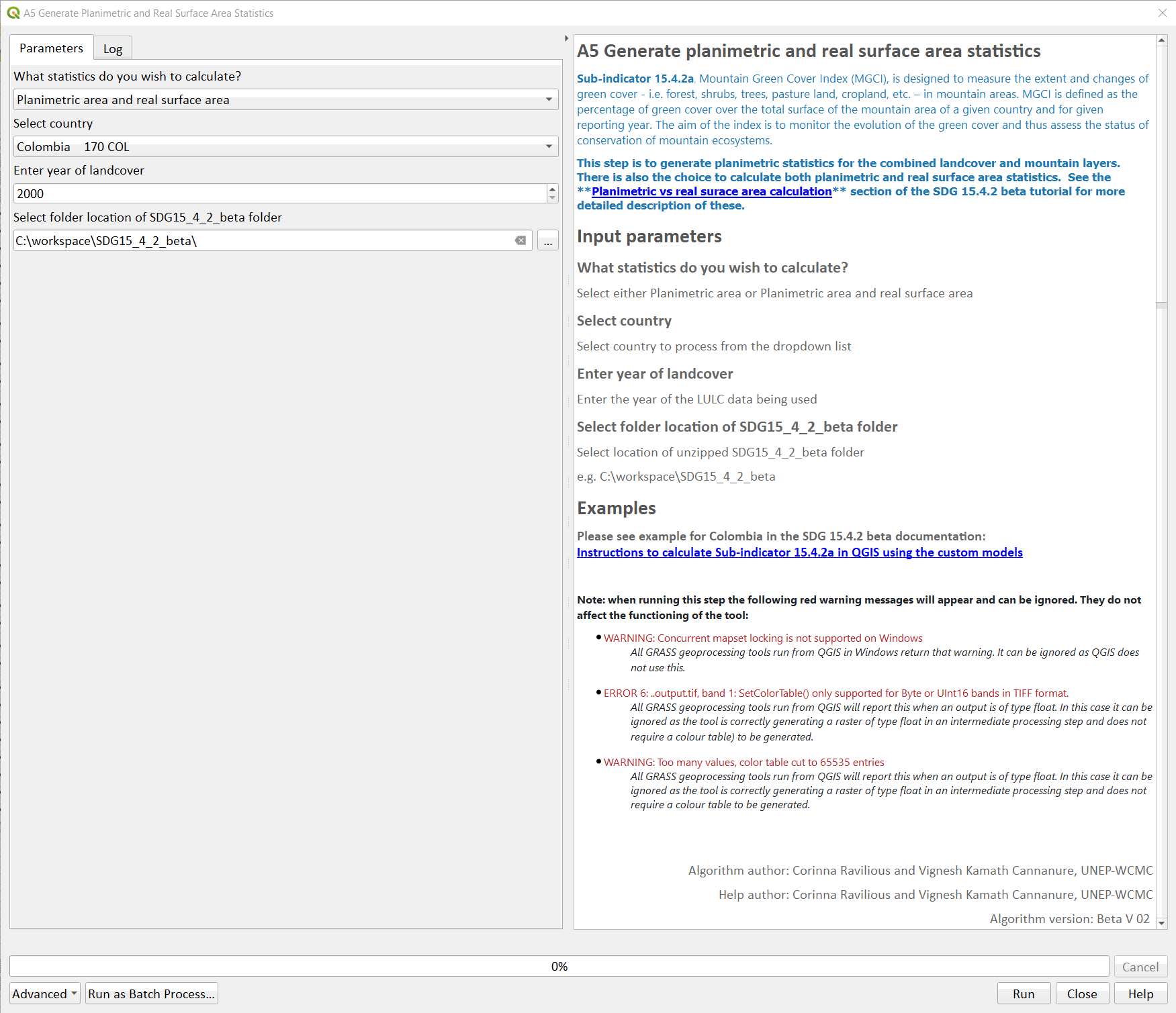
Input parameters
Follow the instructions in the right-hand panel of the tool interface (see screengrab above)
Click Run.
You can run subsequent years by then clicking Change parameters and change the landcover to e.g. the 2015 dataset and year to 2015. Click Run. Repeat this until you have run all the years you wish to run.
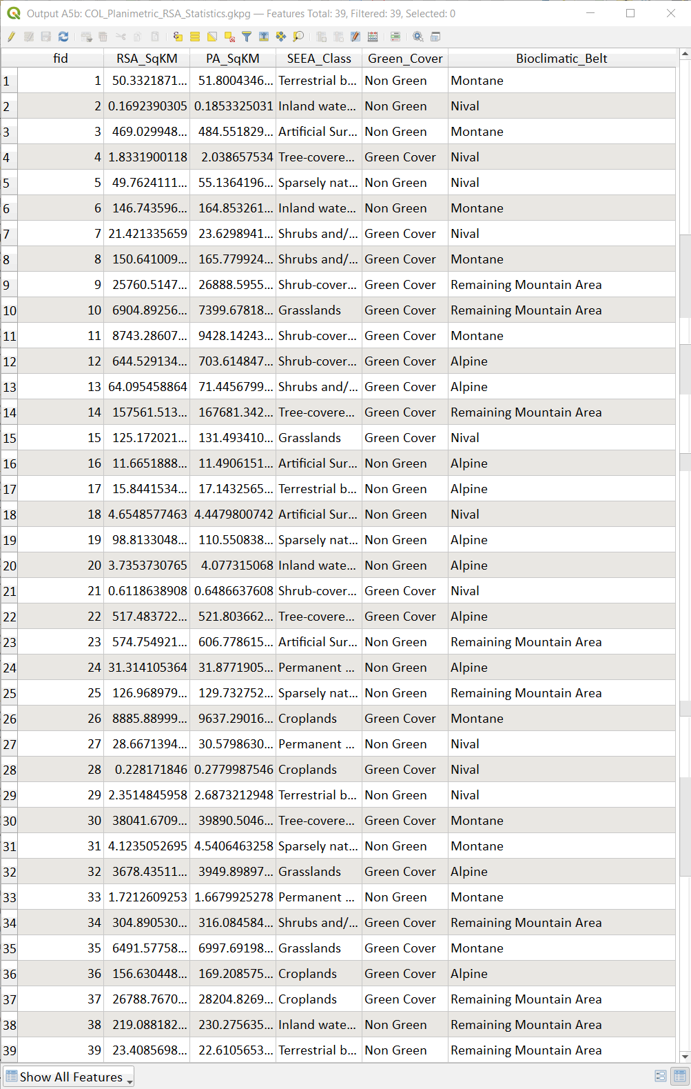
This output is the main statistics table from the analysis, from which other summary statistics tables will be generated:
Note: when running this step the following red warning messages will appear and can be ignored. They do not affect the functioning of the tool:
- WARNING: Concurrent mapset locking is not supported on Windows
All GRASS geoprocessing tools run from QGIS in Windows return that warning. It can be ignored as QGIS does not use this.
- ERROR 6: ..output.tif, band 1: SetColorTable() only supported for Byte or UInt16 bands in TIFF format.
All GRASS geoprocessing tools run from QGIS will report this when an output is of type float. In this case it can be ignored as the tool is correctly generating a raster of type float in an intermediate processing step and does not require a colour table) to be generated.
- WARNING: Too many values, color table cut to 65535 entries
All GRASS geoprocessing tools run from QGIS will report this when an output is of type float. In this case it can be ignored as the tool is correctly generating a raster of type float in an intermediate processing step and does not require a colour table to be generated.
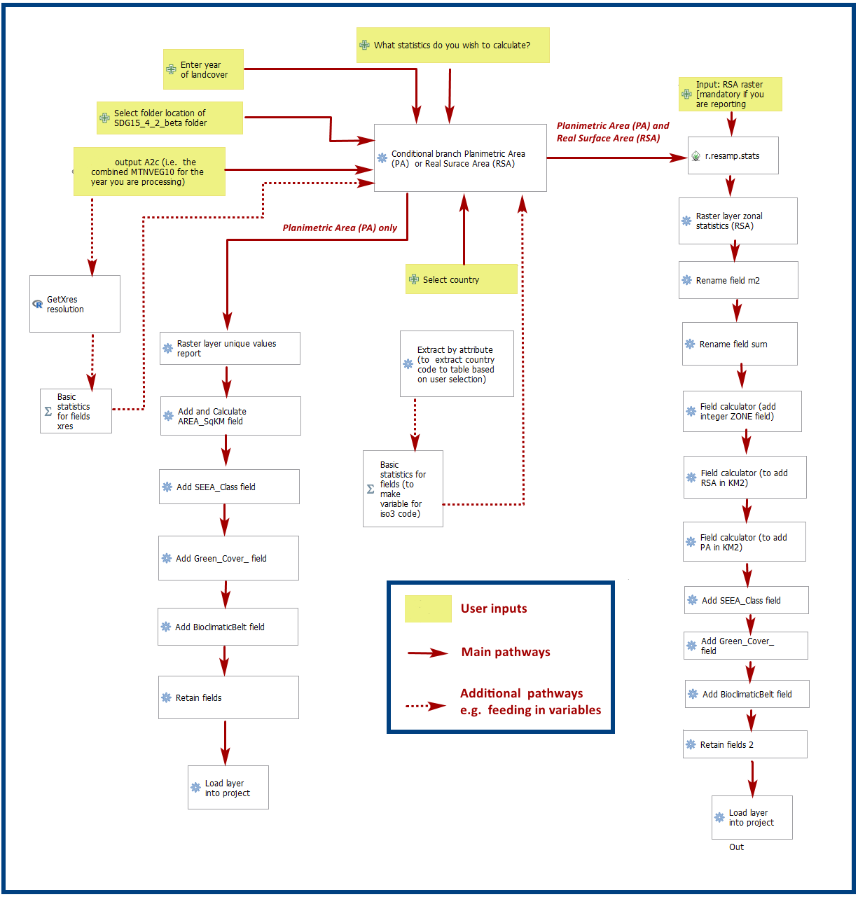
Tool A5 model diagram
Step A6 Formatting to reporting tables#
This statistics table contains the estimates of 15.4.2 sub-indicator a, disaggregated by land cover type. We will remove unwanted fields and calculate the Mountain Green Cover Index estimates. The MGCI is calculated by diving the area of green cover the total area of each bioclimatic belt and the total mountain area and multiplying it by 100.
In the Processing Toolbox, under Models, click on model A6 Formatting to Reporting Tables.
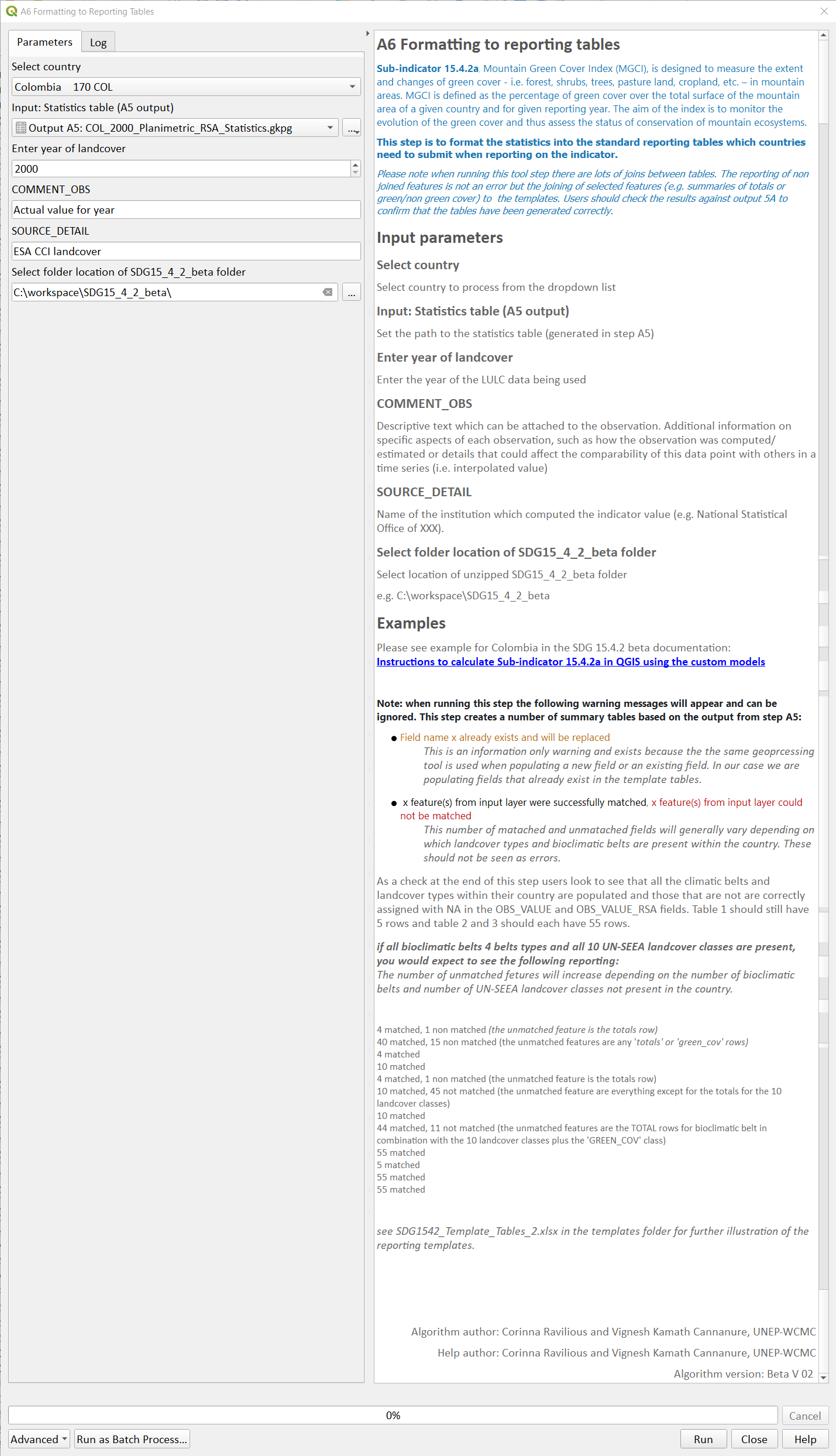
Input parameters
Follow the instructions in the right-hand panel of the tool interface (see screengrab above)
Click Run.
You can run subsequent years by then clicking Change parameters and change the LULC to e.g. the 2015 dataset and year to 2015. Click Run. Repeat this until you have run all the years you wish to run.
If you had landcover for all the reporting years and have run these steps for all the years then Sub-indicator a is now complete, otherwise there is one last interpolation step to interpolate values for the missing years.
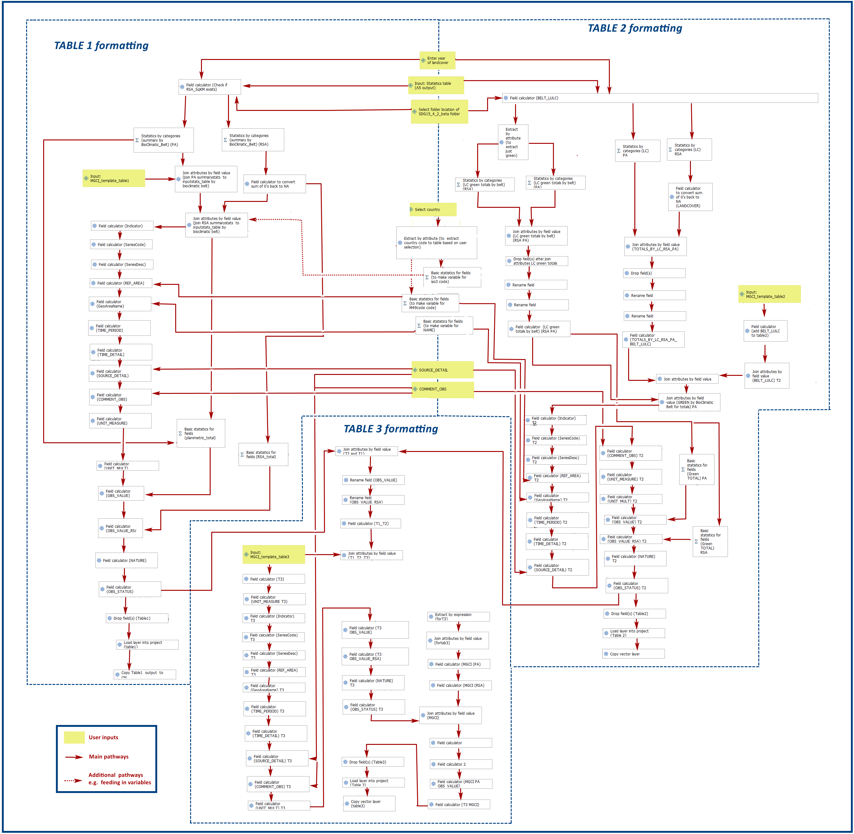
Tool A6 model diagram
Step A7 Interpolation of reporting tables#
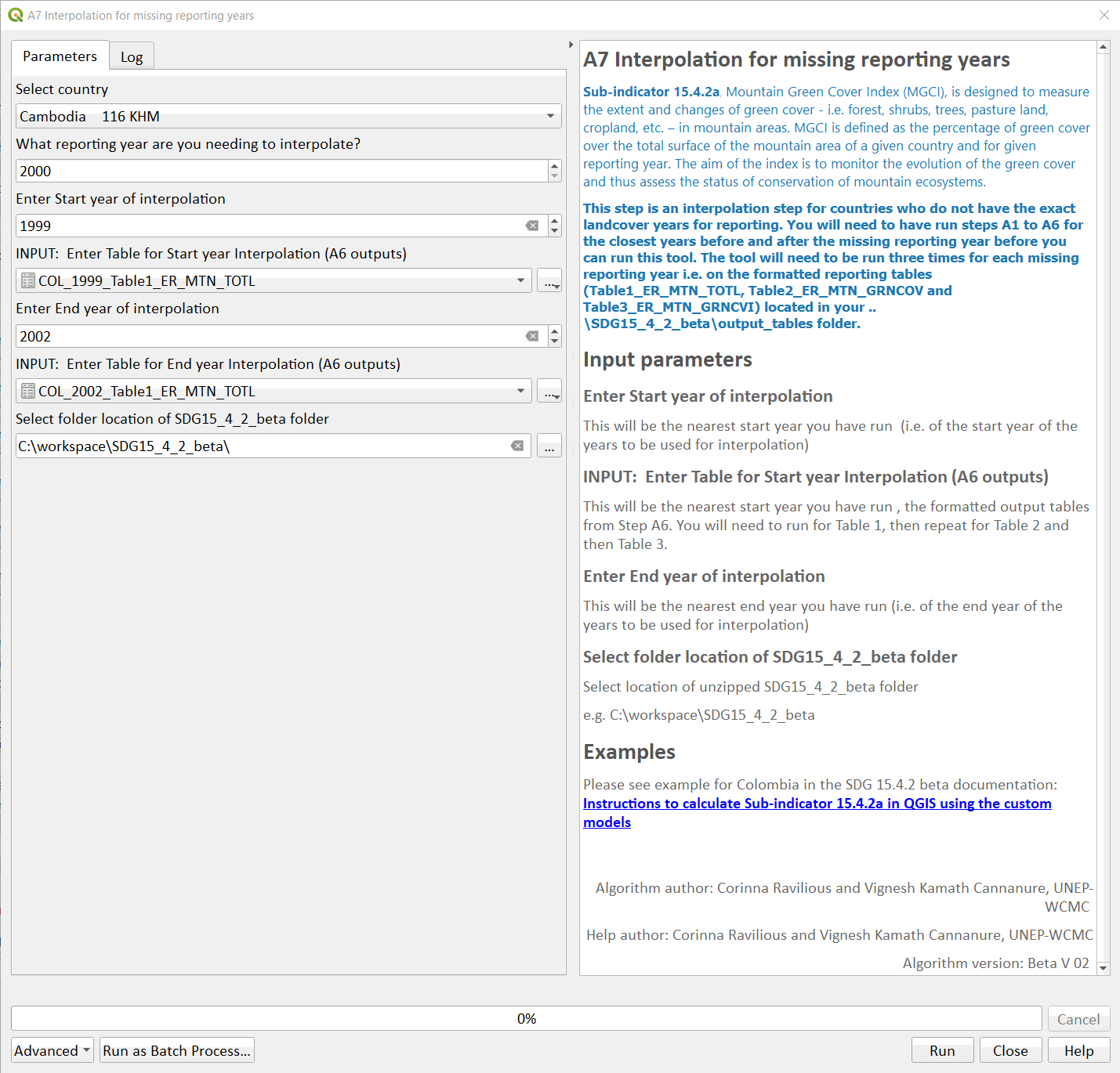
This step is an interpolation step for countries who do not have the exact land cover years for their reporting. You will need to have run steps A1 to A6 for the closest years before and after the missing reporting year before you can run this tool. The tool will need to be run three times for each missing reporting year i.e. on the formatted reporting tables (Table1_ER_MTN_TOTL, Table2_ER_MTN_GRNCOV and Table3_ER_MTN_GRNCVI) located in your ..SDG15_4_2_betaoutput_tables folder.
In the Processing Toolbox, under Models, click on model A7 Interpolation for missing reporting years.
Input parameters
Follow the instructions in the right-hand panel of the tool interface (see screengrab above)
Click Run.
You can run subsequent tables and years by then clicking Change parameters and changing the parameters accordingly. Click Run. Repeat this until you have run for all three reporting tables and for all the missing years you wish to interpolate.
Sub-indicator a is now complete.
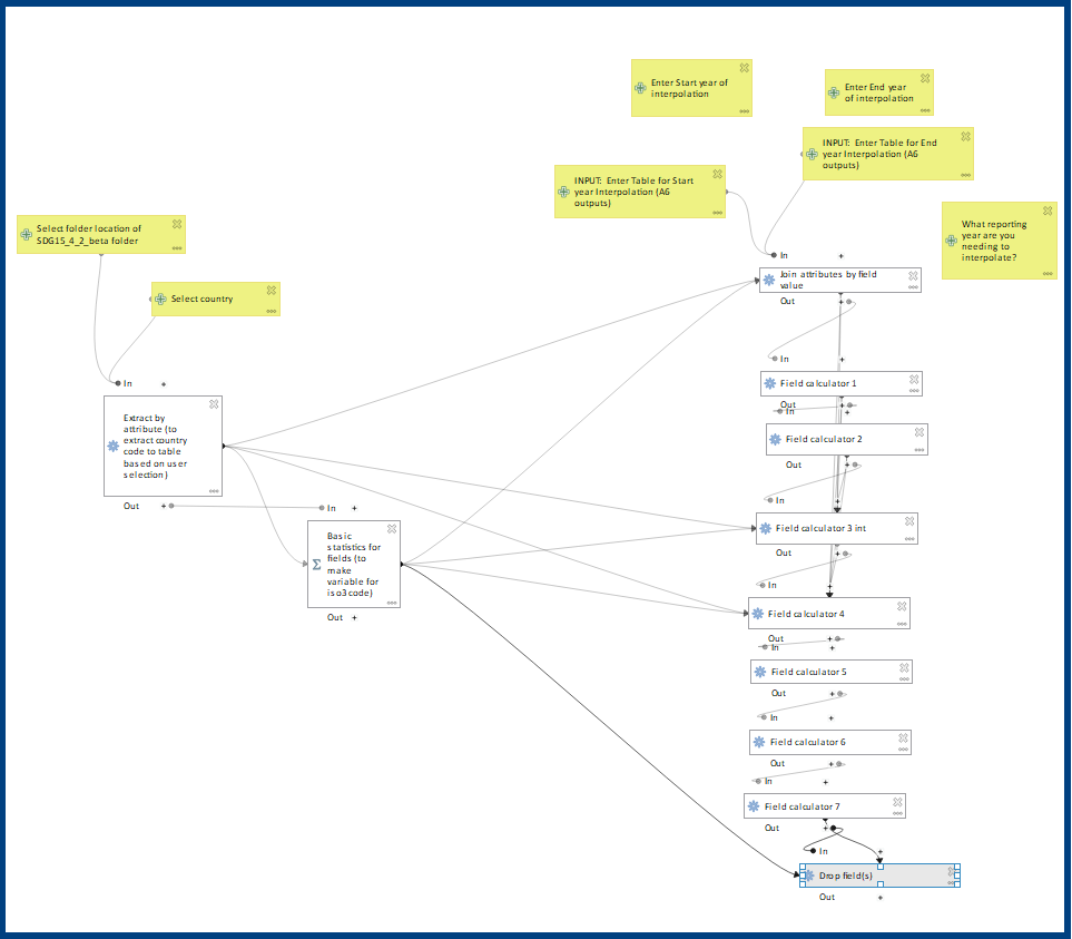
Tool A7 model diagram
Instructions to calculate Sub-indicator 15.4.2b in QGIS using the custom models#
This section of the tutorial explains in detail how to calculate value estimates for sub-indicator 15.4.2b in QGIS, continuing to use Colombia as a case study. Sub-Indicator 15.4.2b is designed to monitor the extent of degraded mountain land as a result of landcover change of a given country and for given reporting year.
As a reminder, in accordance with the SDG indicator’s metadata countries are required to compute estimates for Sub-Indicator 15.4.2b for a baseline for approximately 2000-2015, and subsequently every three years (2018, 2021, 2024, 2027 and 2030). Therefore, for the example in this tutorial we will use the ESA-CCI landcover products for 2000, 2015 (for the baseline) and 2018 (for the reporting year). ESA-CCI land cover data are not yet available beyond 2021 so we have therefore not yet been able to calculate subsequent years in this example.
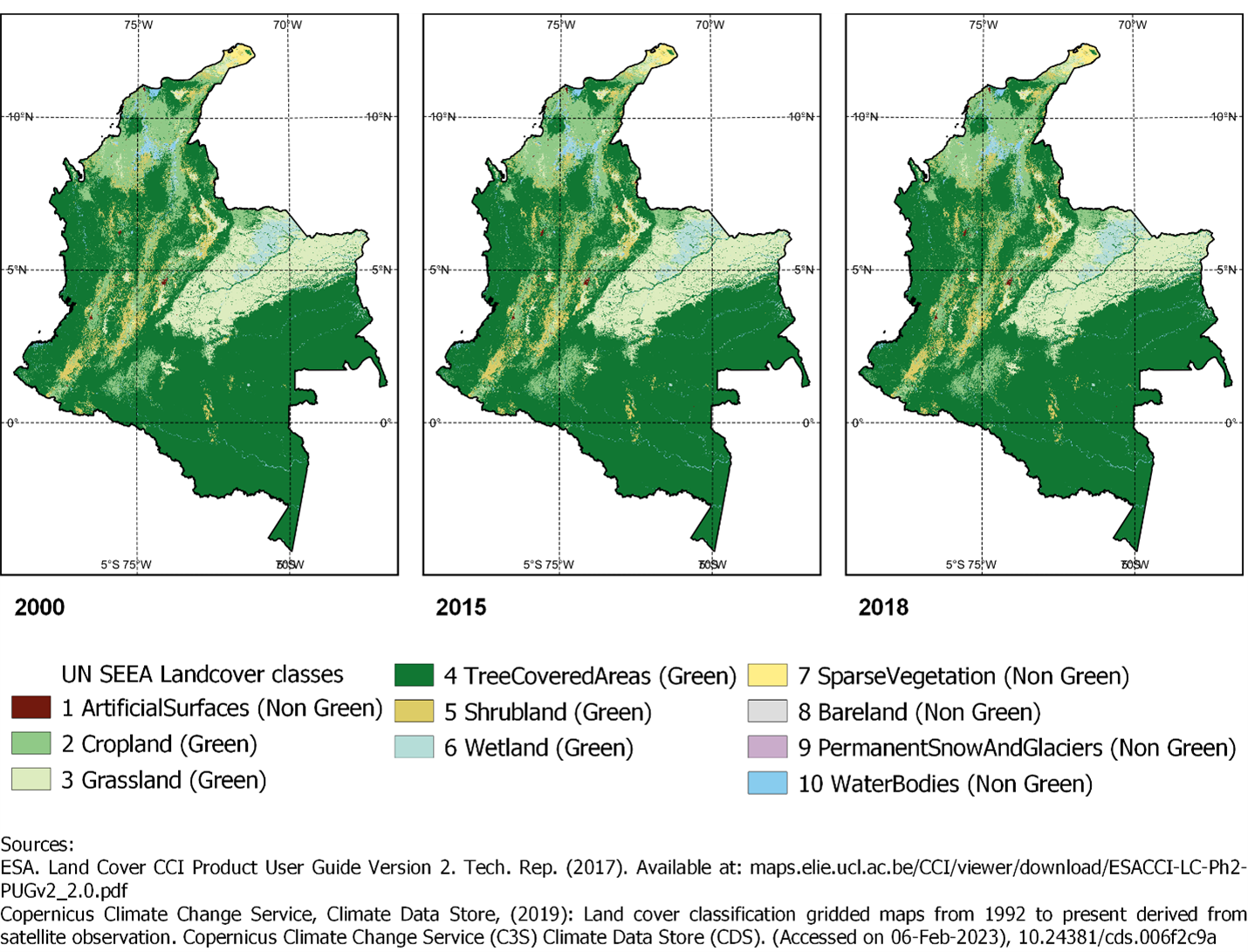
This section of the tutorial assumes that the user has already calculated sub-indicator 15.4.2a and has therefore already downloaded and translated the land cover datasets to UN-SEEA classes for the baseline and reporting years as presented in the figure below.
Landcover reclassified into UN-SEEA classes for 2000, 2015 and 2018
The boundaries and names shown, and the designations used on this map do not imply official endorsement or acceptance by the United Nations.
SGD Indicator 15.4.2b requires us to identify change between LC classes in each reporting period, therefore the first requirement for sub-indicator 15.4.2b is to develop a transition matrix that specifies the land cover changes occurring in a given land unit (pixel) as being either degradation, improvement or neutral transitions. The definition of degradation adopted for the computation of this indicator is the one established by the Intergovernmental Science-Policy Platform on Biodiversity and Ecosystem Services (IPBES).
Countries may choose to either calculate degradation using the default land cover legend for this indicator and default transition matrix provided or from a native or simplified legend of a national land cover dataset if they have the advantage of better representing degradation transitions compared to the broader default transitions.
In this tutorial the default method is described using the default legend and transition matrix, while Annex 2 outlines the additional/alternative steps required to generate a transitions matrix using a nationally adapted land cover legend. In both cases the output results in the same 3 classes (stable, degradation and improving) and both needed to be disaggregated and reported by both land cover transition and bioclimatic belt.
Step B1 Combine land cover datasets#
First, we will generate a single raster containing a value to represent both year 1 land cover and year 2 land cover. We will demonstrate using the default method using the UN-SEEA reclassified landcover rasters in equal area projection that were previously reclassified for the computation of sub-indicator a. As indicated above, users can choose to use the rasters projected to equal area projection containing the full or a simplified national land cover legend if there is a preference/advantage of calculating land cover transitions compared to using the default legend and transition matrix. The processing is the same regardless which method is chosen.
In this example we will use the UN-SEEA reclassified landcover datasets for 2000 and 2015 for the baseline and UN-SEEA classified landcover 2015 to 2018 rasters for the 2018 reporting year. As each dataset has the same landcover values (values 1-10 for UN-SEEA classification) we need to change the values in one of the years to be able to distinguish between classes in year1 and year2. We will multiply year1 landcover classes by 1000 before summing the datasets together. So, for example values for year 1 when using the default legend will range from 1000 – 10000 and values for year 2 will remain 1 -10 and the resultant output will have values ranging from a minimum of 1001 to a maximum of 10010 (depending on which landcover transitions are present).
In the Processing Toolbox, under Models, click on model B1 Combine landcover datasets.
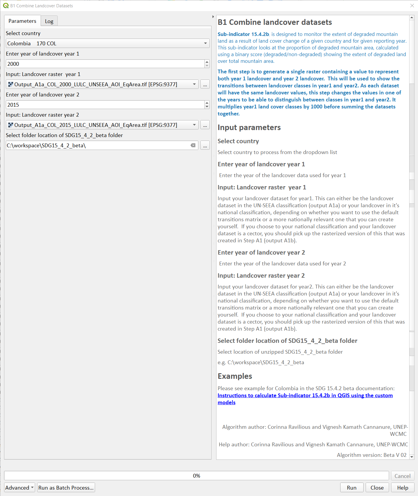
We will calculate the baseline period first i.e., using 2000 land cover (year 1) and 2015 land cover (year 2).
Input parameters
Follow the instructions in the right-hand panel of the tool interface (see screengrab above)
Click Run.
You can run subsequent years by then clicking Change parameters and change the landcover period and datasets to the next reporting period e.g., using 2015 landcover (year 1) and 2018 landcover (year 2). Click Run. Repeat this until you have run all the periods you wish to run.
When using the default UN-SEEA land cover legend, this means that a value of 2001 means a land cover class 2 in year 1 and a land cover class 1 in year 2. A value of 10010 would mean a land cover class 10 in year 1 and a land cover class 10 in year 2. In other words, year 1 is represented by the first digit for values 1 to 9, and by the first 2 digits for land cover class 10. Year 2, on the other hand, is represented by the right hand digit (for values 1-9) and the right hand 2 digits for value 10.
By default the raster will appear with a graded colour ramp. This can be changed by right-clicking on the output dataset and selecting properties>>Symbology and changing the render type from Singleband gray to Paletted/Unique values , then clicking the Classify button. This will show all the unique combinations of landcover 1 and landcover 2 in the combined dataset.
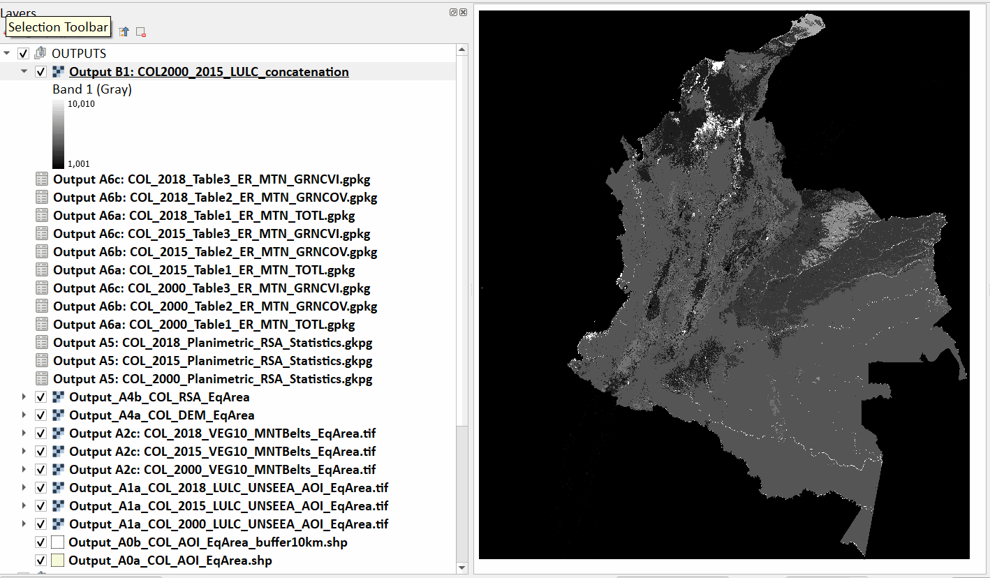
The boundaries and names shown, and the designations used on this map do not imply official endorsement or acceptance by the United Nations.
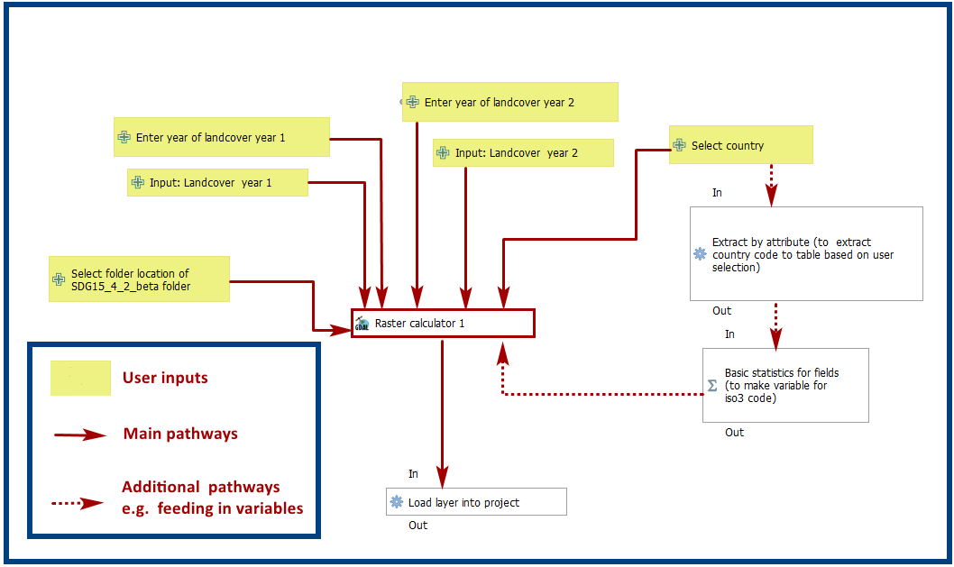
Tool B1 model diagram
Step B2 Generate transition matrix#
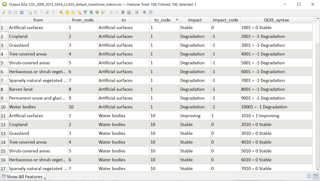
You can either use the default transitions matrix or generate a national one. The default transitions matrix csv file can be downloaded from the GitHub repository showing the unique combination of transitions using the default UN-SEEA classes as presented in the figure below. The default transitions matrix lists the transitions from the landcover classes to the 3 change classes Stable (0), Degradation (-1) and Improving (1).
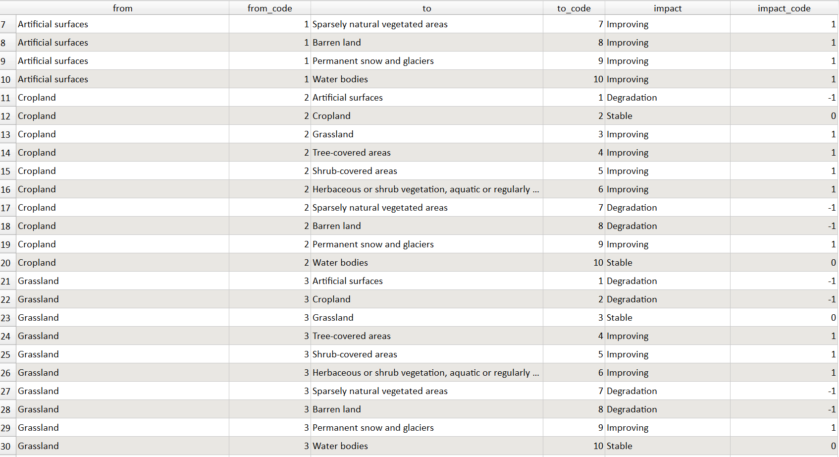
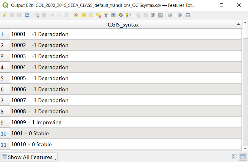
Despite the clarity of this format transitions matrix, the reclassification tools in QGIS require a very specific format for the reclassification table. We therefore need to add an additional field and calculate it to be in the required QGIS syntax. This field will then be saved into a new CSV file which can be used by the QGIS geoprocessing tool.
Note that we are taking the Landcover code for year 1 and multiplying it by 1000 (as described above) and summing it with the land cover code for year 2 before combining it with the rest of the QGIS syntax.
If are using a national land cover transition matrix you can prepare a transitions table in the same format as the default transitions table in Excel or you can generate a csv file from the unique combinations for the land cover types using the combined land cover dataset for the two years. We illustrate this below (the default UN-SEEA classes have been used for illustration purposes only).
In the Processing Toolbox, under Models, click on model B2 Generate Transition Matrix.
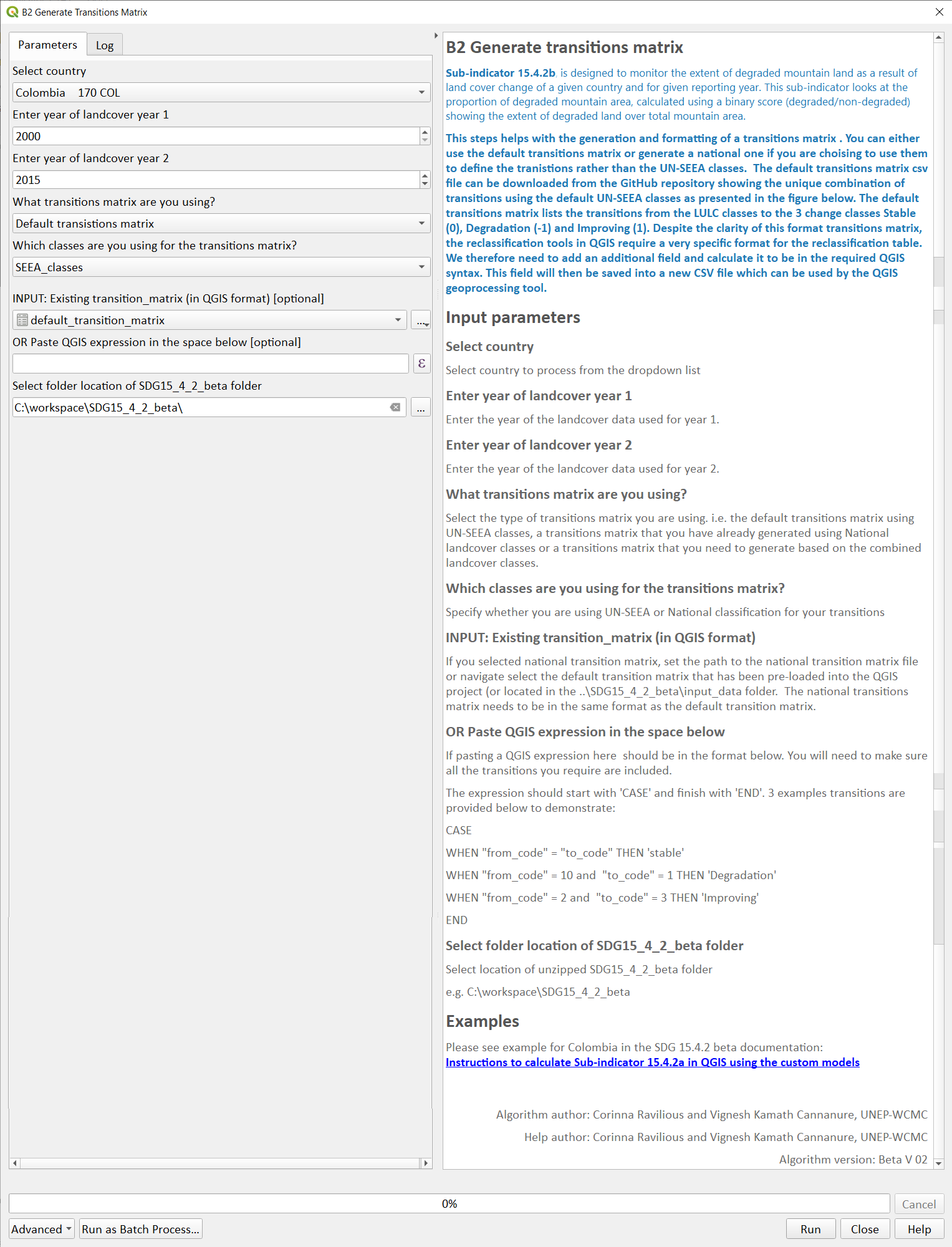
Input parameters
Follow the instructions in the right-hand panel of the tool interface (see screengrab above)
Click Run.
The resultant table should look like this:
*Important Note: Be careful if using this same table for other time periods as it is based on transitions between two specified time periods. E.g., in this case 2000 and 2015. There may be other possible transitions that are not present in this time period but may be possible for other years. Therefore, before using this transitions matrix for other time periods either check for missing entries and manually add them to this table or generate a new transitions table for the new time period.*
Tool B2 model diagram

Step B3 Reclassify land cover transitions to impacts#
The next step is to reclassify the outputs from the combined landcover datasets for year 1 and year 2, first for the baseline period (2000 to 2015) and then for the reporting period (e.g., 2018). We will use the transitions matrix generated in the previous steps. In this example we use the default transitions matrix, but the steps are the same if a national transitions matrix is being used.
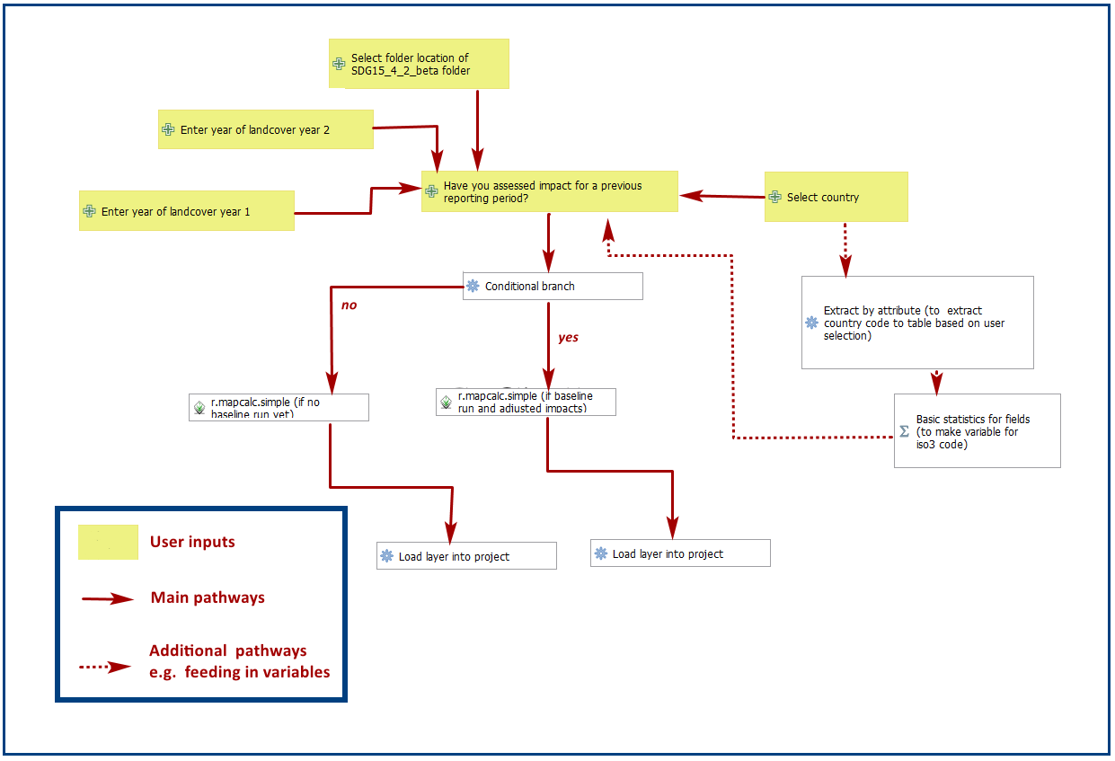
After calculating the baseline reporting period, for assessing the area of degraded mountain land in subsequent reporting periods , the most recent data point of the reference reporting year needs to be compared to the baseline. This means, if we are to calculate the total degraded mountain land for the first reporting year of the Indicator (2018), we would first (1) calculate the area degraded in the baseline period (2000-2015) and then (2) calculate the degraded land in the period 2016 -2018 based on the following the below figure. There is an option in the tool Have you assessed impact for a previous reporting period? which will enable the model to automatically make that adjustment.
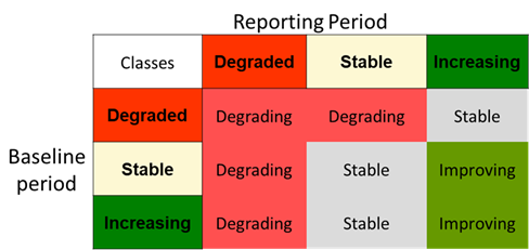
This basically means that area degraded for the reporting period 2018 is calculated by summing : (i) new areas degraded in 2016-2018 period and (ii) areas identified as degraded in the baseline period that remain degraded. If we were to do the same for the next reporting year (2021), we would calculate the degraded land for the 2016 -2021 period, and follow exactly the same approach.
In the Processing Toolbox, under Models, click on model B3 Reclassify landcover transitions to impacts.
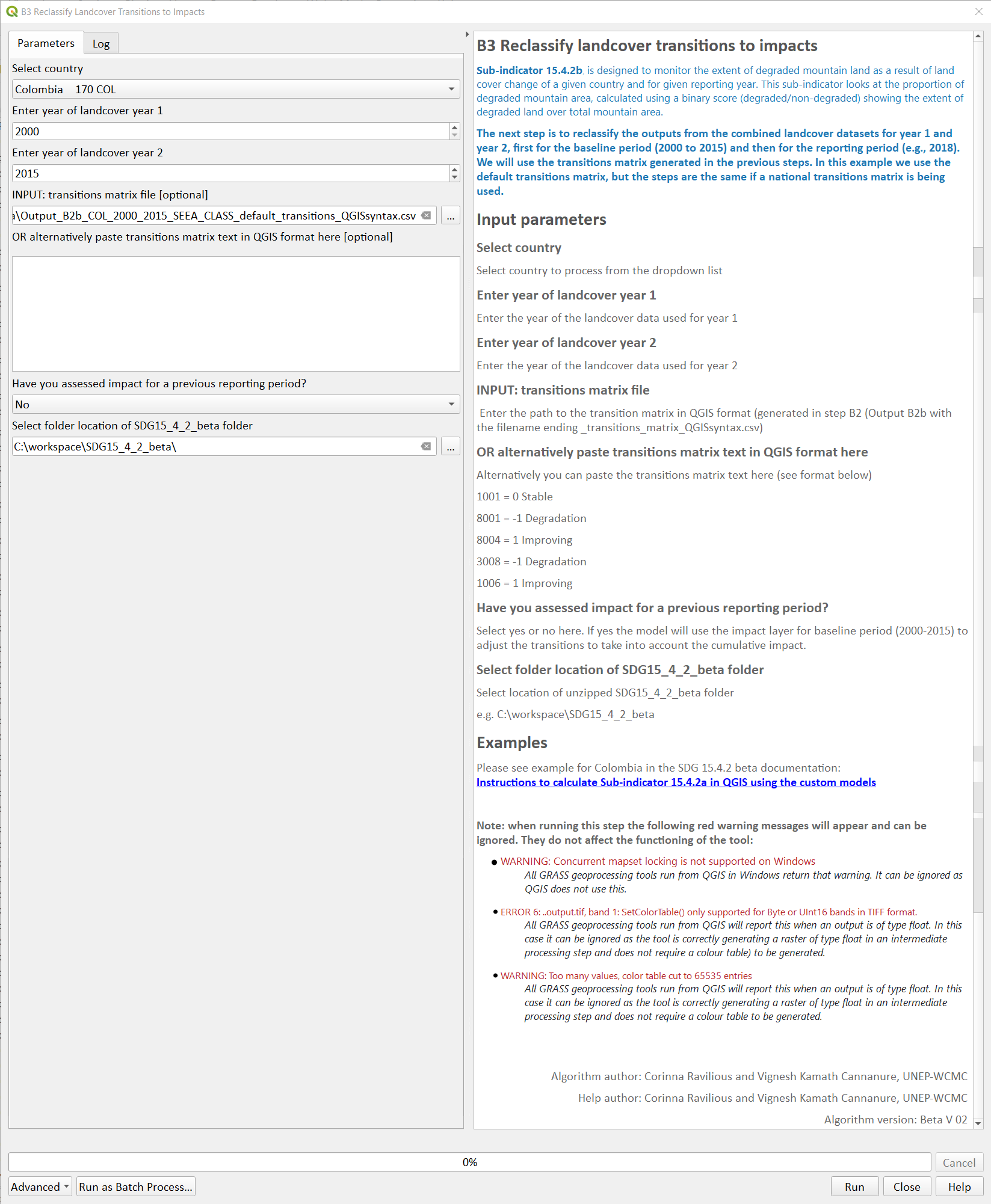
Input parameters
Follow the instructions in the right-hand panel of the tool interface (see screengrab above)
Click Run.
Repeat the above step for the next reporting period i.e., using 2015 landcover (year 1) and 2018 landcover (year 2)
You can ignore the two warning messages that appear in red– these do not affect the correct generation of the outputs.
WARNING: Concurrent mapset locking is not supported on Windows
ERROR 6: C:workspaceMGCIoutputsUNSEEA_LULC2000_2015_EqArea_reclassed_impact.tif, band 1: SetColorTable() only supported for Byte or UInt16 bands in TIFF format.
The resultant map should show should show the three impact categories:
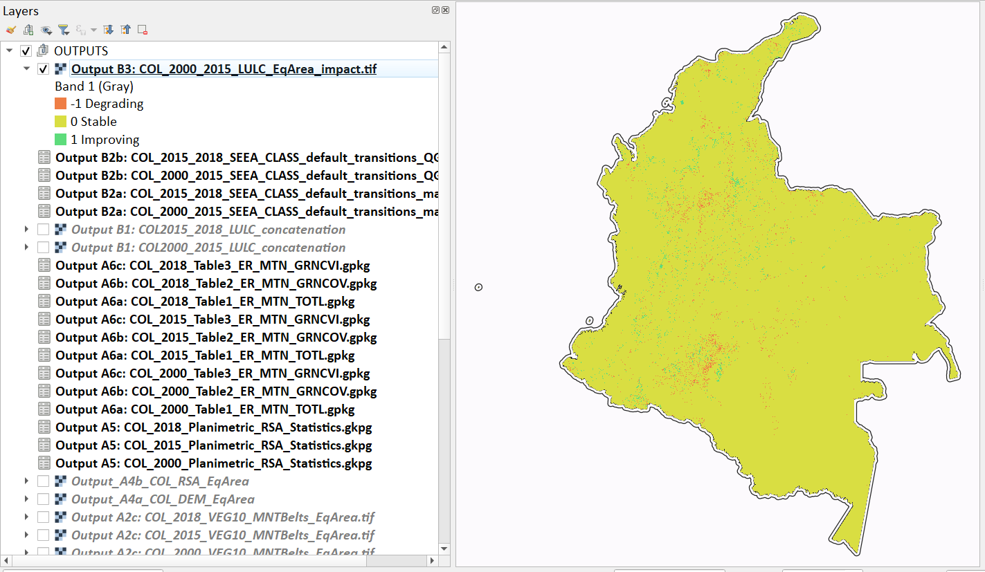
The boundaries and names shown, and the designations used on this map do not imply official endorsement or acceptance by the United Nations.
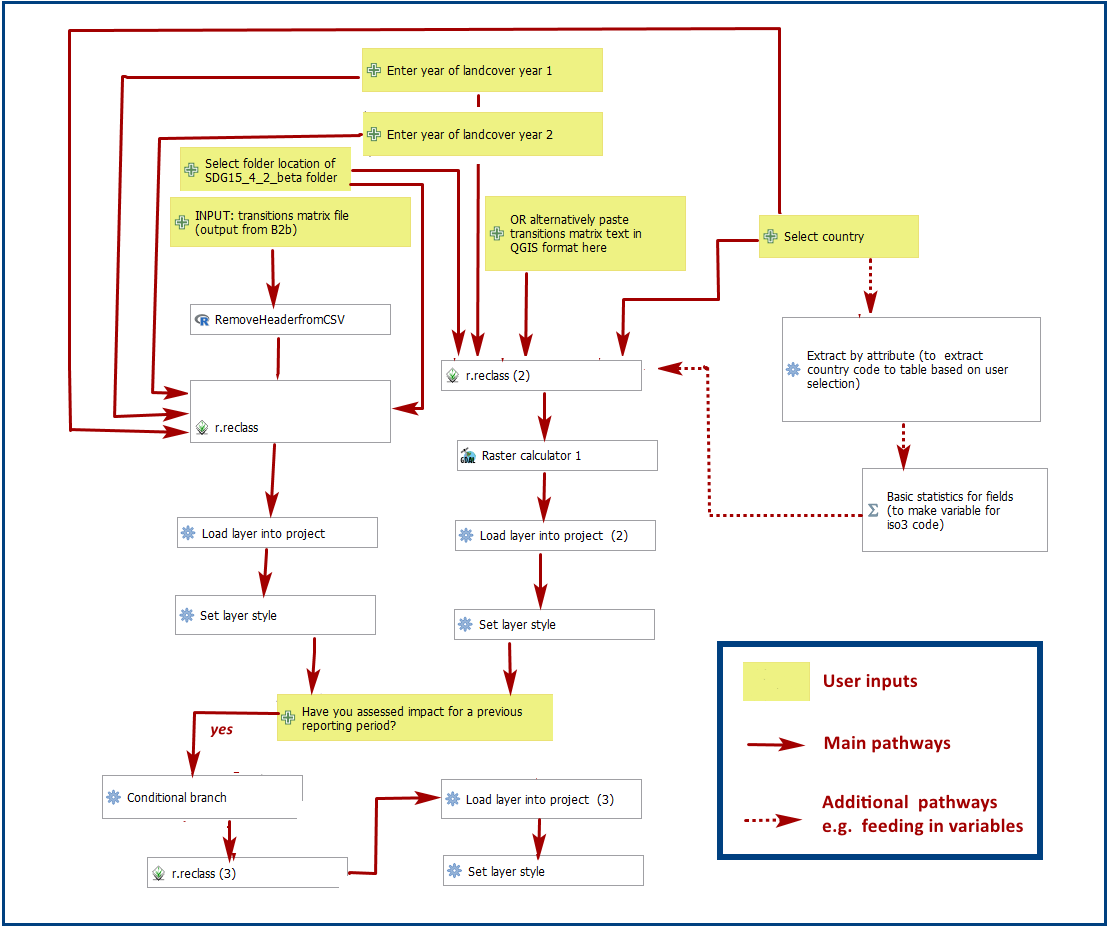
Tool B3 model diagram
Step B4 Combine Bioclimatic belts, land cover transitions and impact layers#
We now have all the layers we need for generating statistics. To make it easier we will again sum the layers together using different factors to change the values in some of the datasets. We have the following datasets which we need to combine to generate the proportion of degraded mountain area disaggregated by land cover transitions, impact status and bioclimatic belt:
Land cover transitions (which in our case using have values 1001-10010 where land cover for year 1 has already been multiplied by 1000 and summed with year 2 values)
We will leave these landcover transitions dataset values as they are.
Bioclimatic belts (which have values 1-4 representing the 4 bioclimatic belts)
We will multiply the bioclimatic belts by 100,000.
Land cover transition impact status (values -1, 0 and 1)
We will change the impact status by adding 2 to each of the values and multiplying by 1,000,000 thus changing values -1 to 1,000,000 (degradation), 0 to 2,000,000 (stable) and 1 to 3,000,000 (improving)
In the Processing Toolbox, under Models, click on model B4 Combine Bioclimatic Belts, land cover transitions and impact layers.
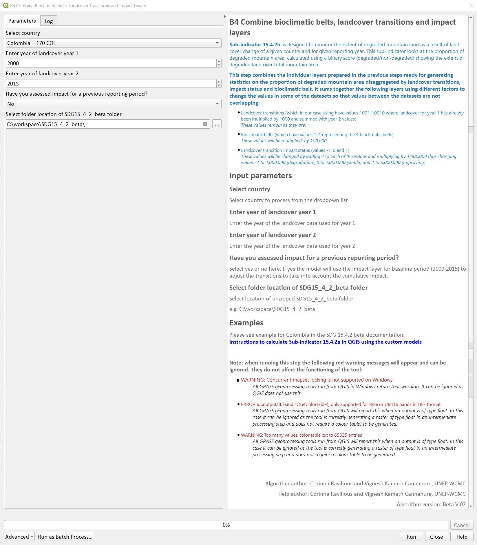
Input parameters
Follow the instructions in the right-hand panel of the tool interface (see screengrab above)
Click Run.
Repeat the above step for the next reporting period i.e., using 2015 landcover (year 1) and 2018 landcover (year 2).
The resultant map should look similar to the image below. Remember that we used various multiplication factors to distinguish between the layers we were combining so they shoud have some very high values.
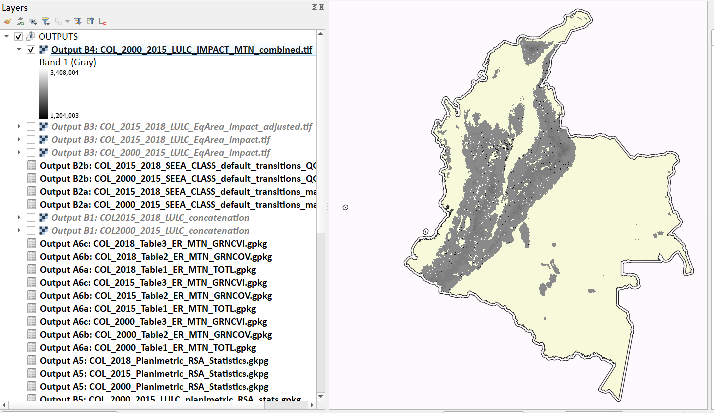
The boundaries and names shown, and the designations used on this map do not imply official endorsement or acceptance by the United Nations.
Tool B4 model diagram
Step B5 Generate planimetric and real surface area statistics#
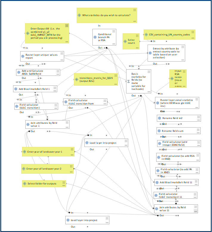
The data are now combined and in a format that we can use to generate the statistics required for the sub-indicator 15.4.2b reporting. The Raster layer unique values report tool will automatically calculate planimetric and real surface area statistics in the output and contain all the disaggregation we require. This output is the main statistics table from the analysis, from which other summary statistics tables will be generated.
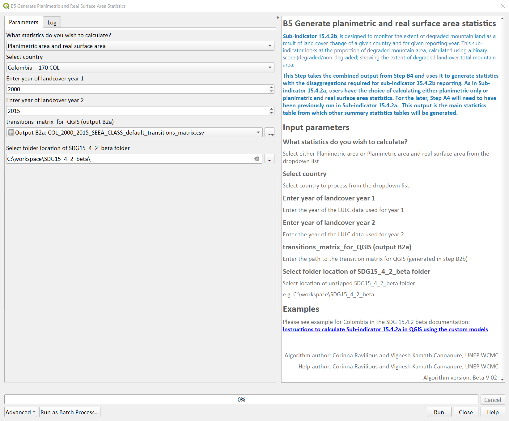
In the Processing Toolbox, under Models, click on model B5 Generate Planimetric and Real Surface Area Statistics.
Input parameters
Follow the instructions in the right-hand panel of the tool interface (see screengrab above)
Click Run.
The resultant table should look similar to the image below:

Tool B5 model diagram
Step B6 Formatting to reporting tables#
This statistics table contains the estimates of 15.4.2 sub-indicator b. We will remove unwanted fields and calculate the Mountain Green Cover Index estimates.
In the Processing Toolbox, under Models, click on model B6 Formatting to Reporting Tables.
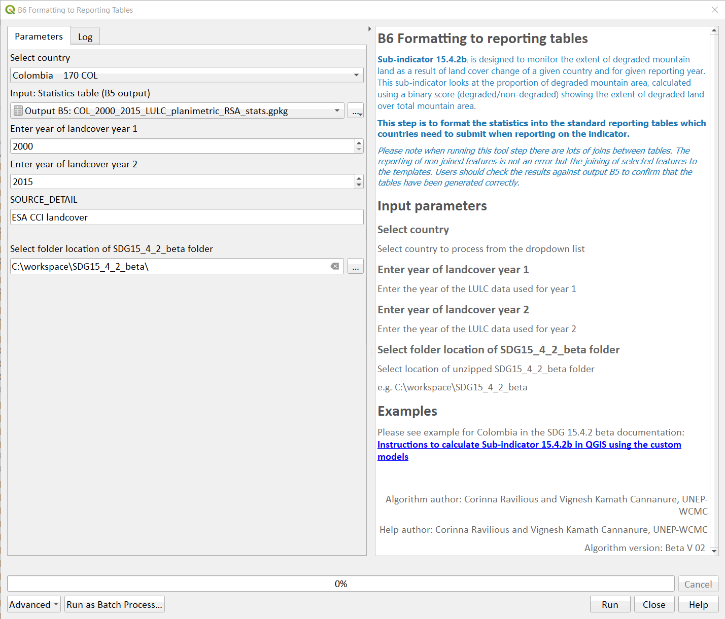
Input parameters
Follow the instructions in the right-hand panel of the tool interface (see screengrab above)
Click Run.
Repeat the above step for the next reporting period i.e., using 2015 landcover (year 1) and 2018 landcover (year 2) and any other reporting periods.
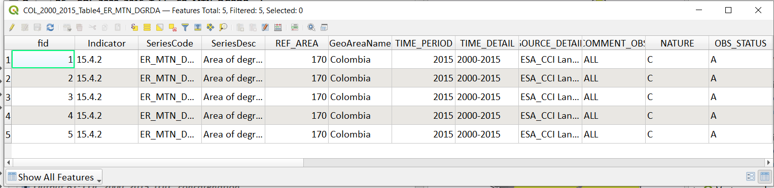
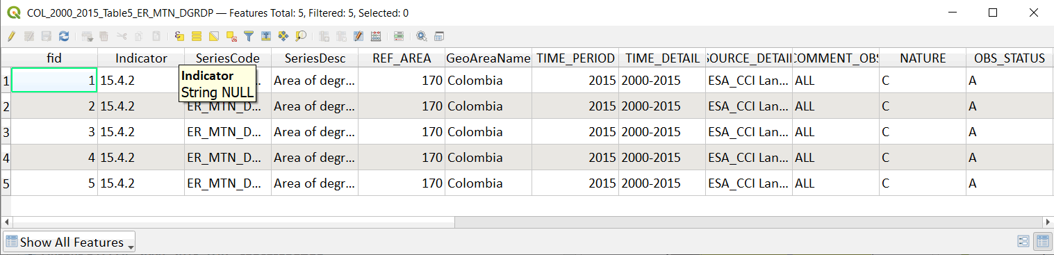
The resultant tables should look similar to the images below:
Tool B6 model diagram