Annex 2

Manual steps to calculate Sub-indicator 15.4.2a in QGIS

This section of the tutorial explains in detail how to calculate value estimates for sub-indicator 15.4.2a in QGIS, using Colombia as a case study. This section assumes that the user has already downloaded the global mountain map made available by FAO to compute this indicator and a land cover dataset meeting the requirements described in section 3.2.

Step-by-step equivalent of Tool step A0: Prepare country boundary and buffer to 10km

The following steps are covered by this tool:

Define projection and buffer country boundary

The first step is to define the projection and an Area of Interest (AOI) for the analysis. The AOI should go beyond the country boundary as outlined in the Defining analysis environments section of the tutorial.

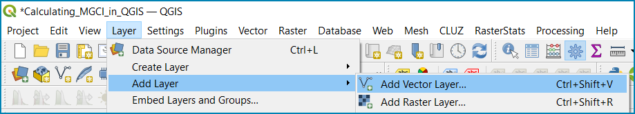
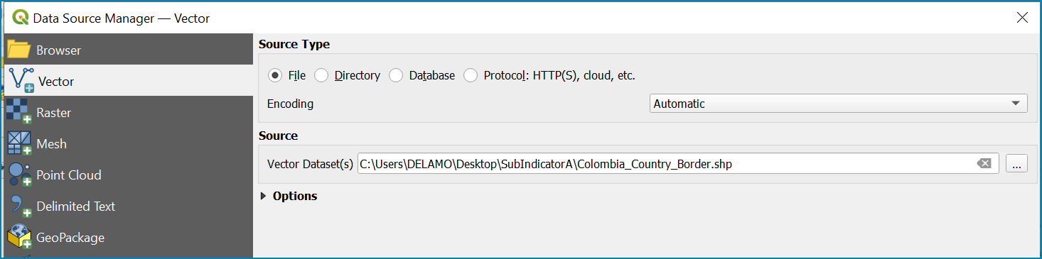
• Add a country boundary layer to QGIS Layer>>Add Layer>>Add Vector Layer

The boundaries and names shown, and the designations used on this map do not imply official endorsement or acceptance by the United Nations.

• Click Add and Close to close the Data Source Manager: Vector dialogue window

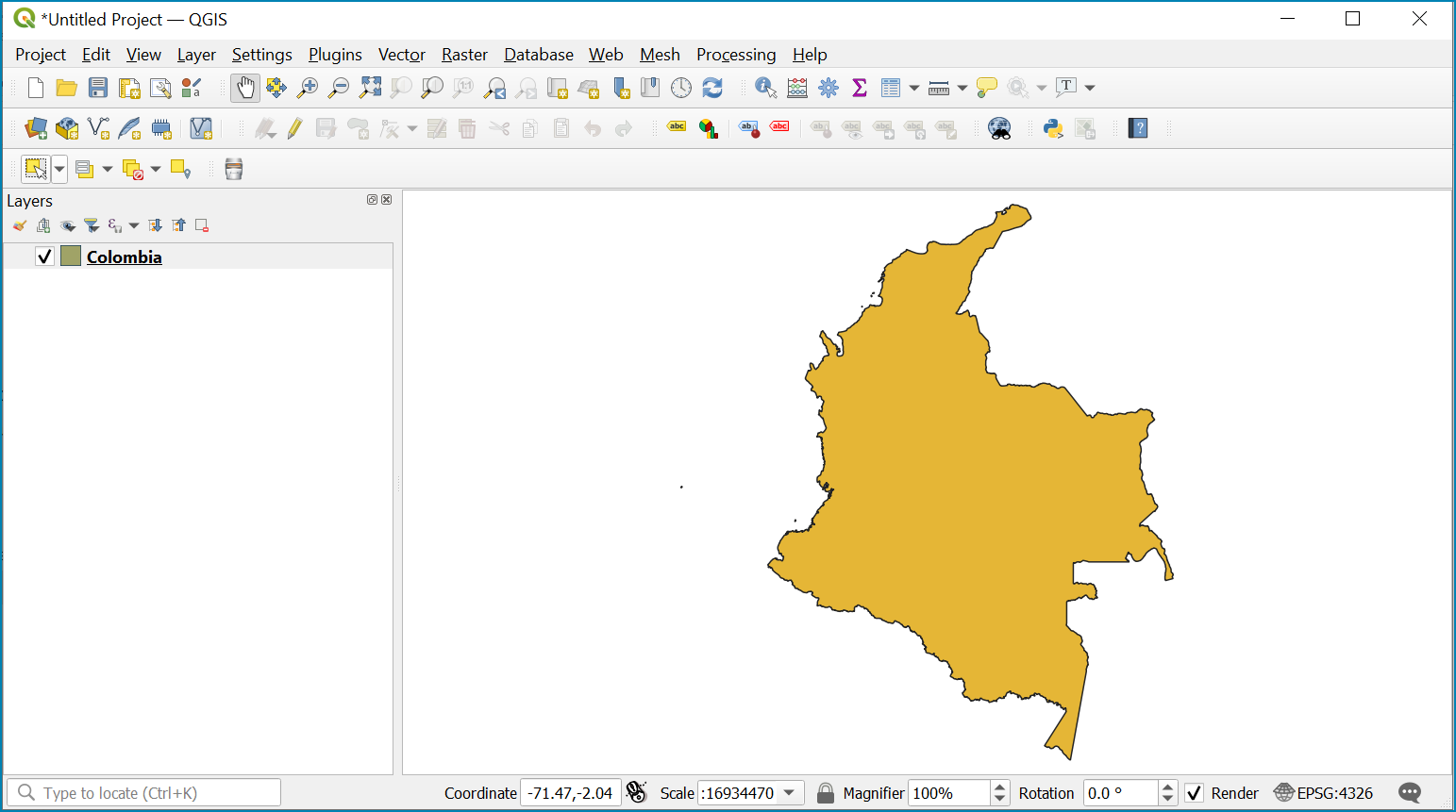
• Right-click on the country boundary layer and click Zoom to Layer

In this example, the boundary layer is in Geographic coordinate system (EPSG 4326). At this stage we want to set-up the projection for the main parts of the analysis. We therefore want to set the project window to an equal area projection and physically project the country boundary to the same projection.

Colombia does have a National Projection that preserve both area and distance (see here) and therefore could be used as a custom projection. In case a national projection that minimize area distortion does not exist for a given country, it is recommended to define a custom Equal Area projection centered on the country area following the instructions described here under ‘’Define projection and generate AOI’’).

Once you have defined the projection to use in the analysis, change the projection set for the QGIS project to your chosen projection. In this example it is the national projection for Colombia.

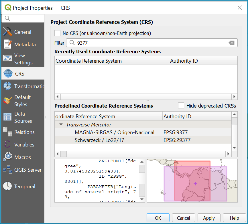
• Click on the project projection EPSG: 4326 in the bottom right hand corner of your QGIS project

• In the Project Properties dialogue window search for the chosen projection in the Filter tab, in this case the projection EPSG 9377

The boundaries and names shown, and the designations used on this map do not imply official endorsement or acceptance by the United Nations.

• Once located click on the chosen projection to set your QGIS project to be displayed in the chosen projection.

• Click Apply and **OK **

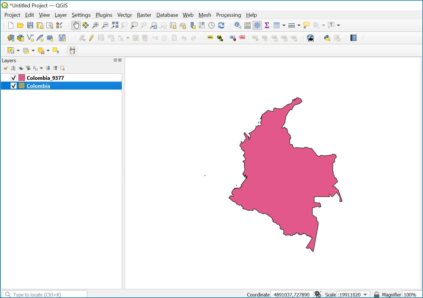
See that the project now displays the custom projection in the bottom right hand corner.

Next use the reproject tool to project the country boundary layer to the 9377 projection

• In the processing toolbox search for the Reproject tool

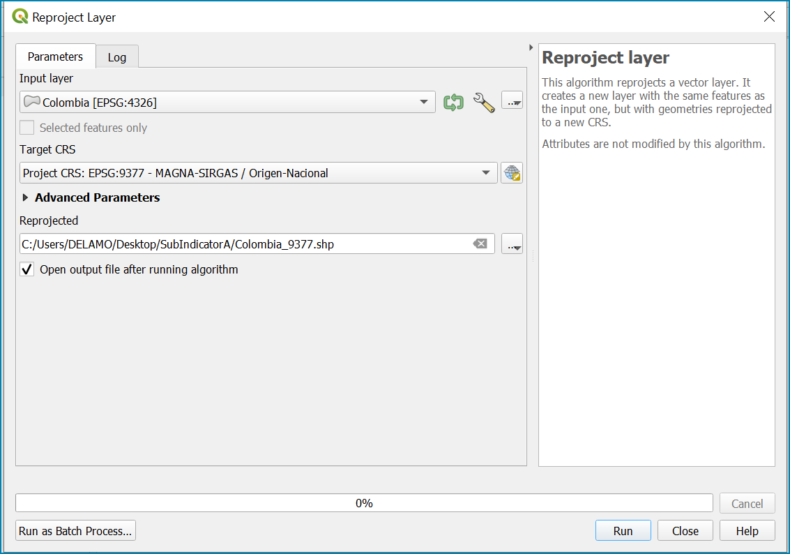
• Set the Input layer to be the country boundary

• Set the Target CRS to be the Project CRS (i.e. the EPSG 9377 projection)

• Set the output name to be the same as the input with a suffix to indicate the projection e.g. in this example **Colombia_9377. **

The boundaries and names shown, and the designations used on this map do not imply official endorsement or acceptance by the United Nations.

Now that the country boundary is in the chosen projection, we can generate the mountains and land cover maps for Colombia.

Step-by-step equivalent of Tool step A1: Prepare and reclassify LULC dataset into UN-SEEA classes

The following steps are covered by this tool:

To demonstrate the steps for processing a raster LULC dataset we will use the Global ESA CCI LULC dataset. If you are using a national dataset, you can skip the following step.

Clip and project LULC raster

The ESA CCI LULC dataset is provided in netcdf (.nc) format. Similarly to Geotiffs, these can be added directly to QGIS.

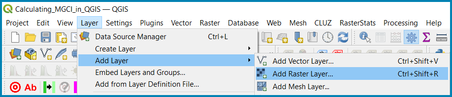
• From the QGIS main toolbar click on Layer>>Add Layer>>Add Raster Layer to add the LULC file to your QGIS session.

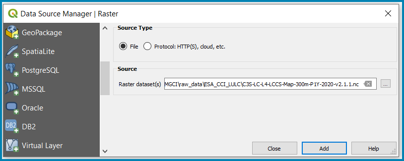
• Click Add

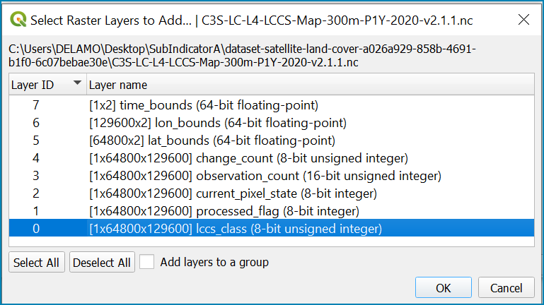
For most formats this will add the LULC dataset to the QGIS session. The Global ESA CCI LULC netcdf file however contains 7 different layers (similar to bands in an image) and users need to select the lccs_class layer.

• Click lccs_class to select the LULC layer

• Click OK and the LULC layer will be added to your QGIS project

• Click Close to close the Data Source Manager: Raster dialogue window

Next check that the LULC layer has correct projection information and appears in the correct place in the QGIS project.

• First check that the LULC layer is correctly overlaying the country boundary data. If it does not your country boundary and/or your LULC layer may be lacking projection information or have the wrong projection information.

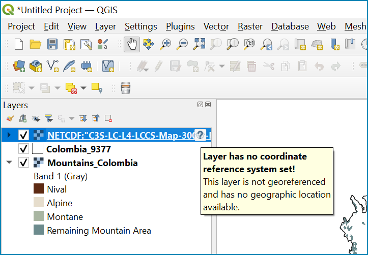
• QGIS will display a ‘’?’’ next to the layer if projection information is missing.

• If projection information is missing define the projection using the Define Shapefile projection tool in the processing toolbox (this will permanently attach projection information to the layer) alternatively you can just define it within the current QGIS project by right clicking on the layer.

In this example we know the LULC is in Geographic coordinate system so we can assign coordinate system EPSG 4326 to the layer

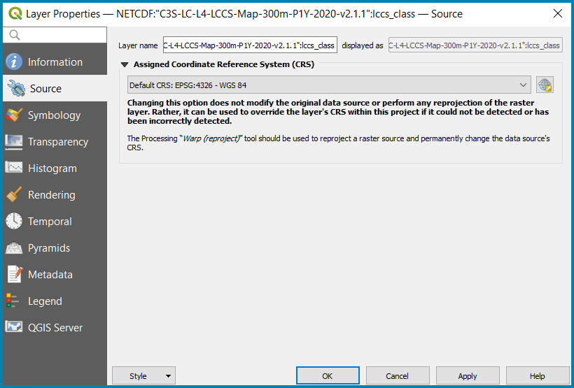
• This layer should now draw correctly on the country boundary.

If the LULC dataset is a regional or global extent it will need projecting and clipping to the AOI.

In this example we are using a global dataset so we will need to clip the raster and save it in the equal area projection.

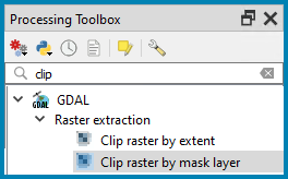
• In the processing toolbox search for Clip

• Double click on the Clip raster by mask layer under the GDAL toolset

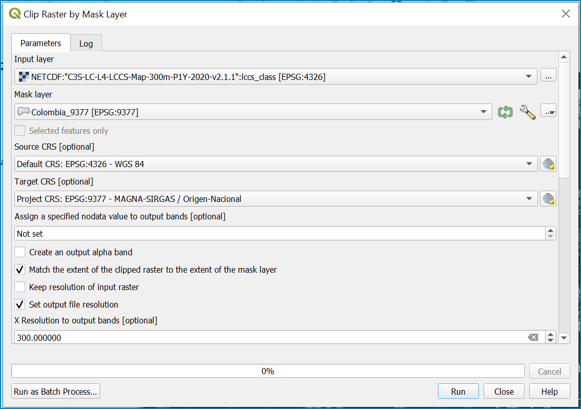
• Select the LULC dataset for the input layer

• Select the national border of the country for the Mask Layer

• Select the Project CRS for the Target CRS

• Tick Match the extent of the clipped raster to the extent of the mask layer

• Tick set the output file resolution

• Type the X and Y resolution in metres (in this case the resolution of the LULC dataset is 300)

• Tick Use Input Layer Data Type

• Set the output Clipped (mask) e.g. to LULC_2020_Colombia.tif (see screengrab below)

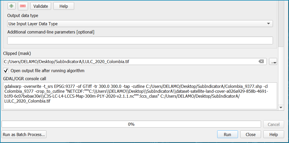
• Click Run to run the tool

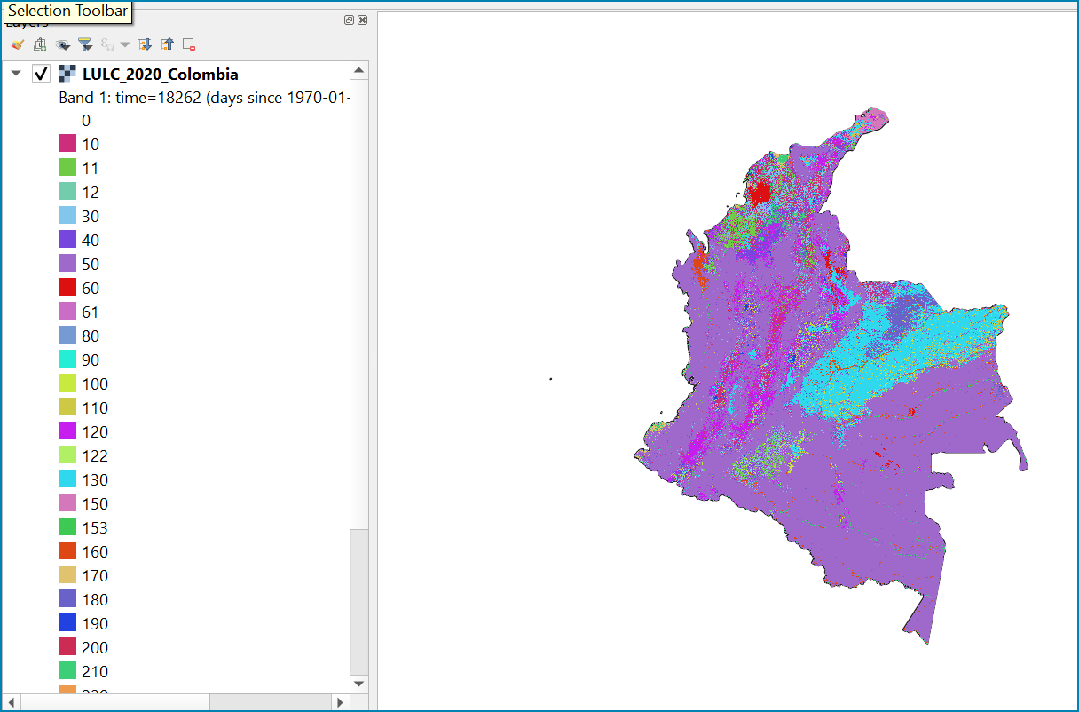
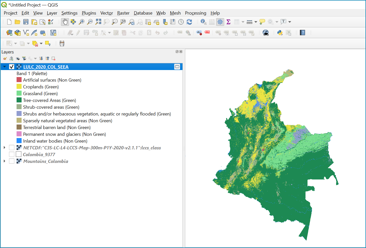
The new clipped LULC dataset in the equal area projection should be added should be added to the map canvas . LULC_2020_Colombia layer) and click properties>>Symbology

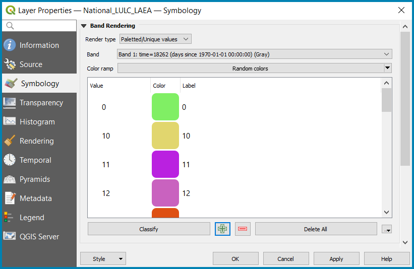
• Change the render type to Palleted/Unique Values

• Click Classify and then OK

You should now see the unique LULC classes present within the AOI for the country.

The boundaries and names shown, and the designations used on this map do not imply official endorsement or acceptance by the United Nations.

Reclassify to UN-SEEA land cover classes

The next step is to reclassify the LULC map into the 10 UN-SEEA classes defined for SDG Indicator 15.4.2

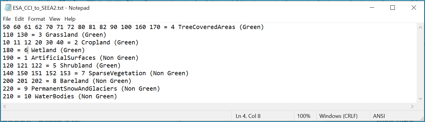
QGIS provides several tools for reclassification. The easiest one to use in this instance is the r.reclass tool in the GRASS toolset as it allows the upload of a simple crosswalk textfile containing the input LULC types on the left and the UN-SEEA reclass values on the right.

• Create a text file to crosswalk landuse/landcover (LULC) types from the ESA CCI or National landcover dataset to the 10 UN-SEEA landcover classes

• Search for reclass in the processing toolbox

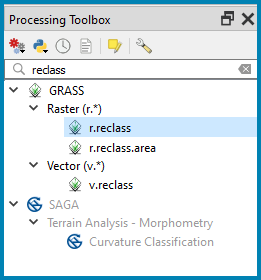
• Double click on r.reclass

• Select the LULC output as the input raster layer

• Set the GRASS GIS region extent to be the same as the input layer

• Set the Reclassified output e.g. VegetationDescriptor_Colombia.tif

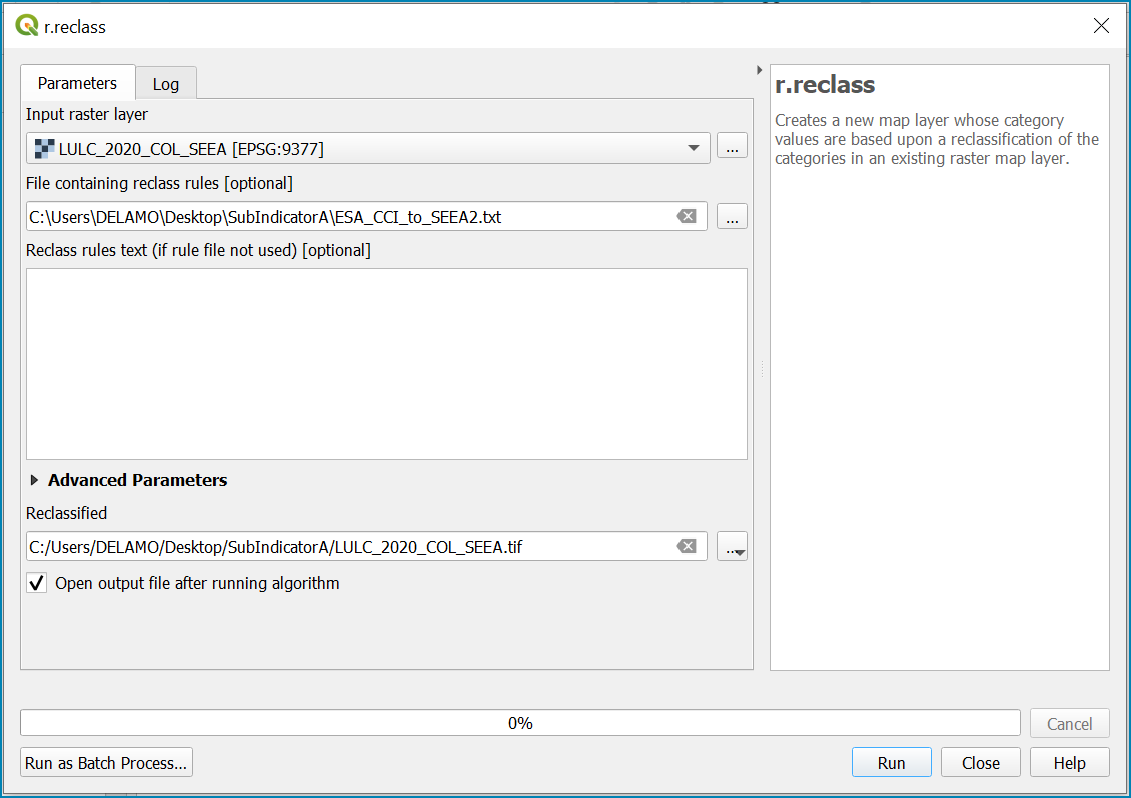
• Click Run to run the tool. The new VegetationDescriptor layer is added to the map.

Although the reclassification only had 6 output classes the symbology initially show values 0-255. This is a QGIS visualisation only and you can see that the actual layer only has 10 values.

• Right click on the layer properties>>>Symbology

• Change the Render type to Palleted Unique values and click Classify to see only the classes present in the raster (i.e. the 1-10 Vegetation descriptor classes) and rename the classes following the UN-SEEA terminology. Give each class a distinctive and identifiable colour.

The boundaries and names shown, and the designations used on this map do not imply official endorsement or acceptance by the United Nations.

Step-by-step equivalent of Tool step A2 Prepare mountains and combine with LULC

The following steps are covered by this tool:

Generate the mountain map for the chosen country

The development of mountain map consists in clipping and reprojecting the SDG 15.4.2. Global Mountain Descriptor Map developed by FAO to area of interest, in this case, the national border of Colombia.

Clip and project global mountain map

From the QGIS main toolbar click on Layer>>Add Layer>>Add Raster Layer to add the global mountain map file to your QGIS session.

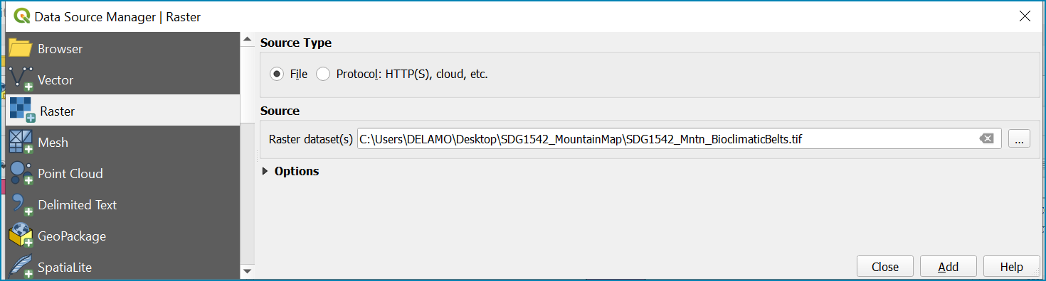
• Click Add

The boundaries and names shown, and the designations used on this map do not imply official endorsement or acceptance by the United Nations.

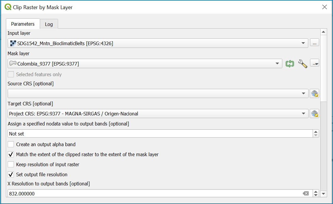
• In the processing toolbox search for Clip

• Double click on the Clip raster by mask layer under the GDAL toolset

• Select the global mountain descriptor map for the Input Layer

• Select the national border of the country for the Mask Layer

• Select the Project CRS for the Target CRS

• Tick Match the extent of the clipped raster to the extent of the mask layer

• Tick set the output file resolution

• Type the X and Y resolution in metres (in this case 832)

• Tick Use Input Layer Data Type

• Set the output Clipped (mask) e.g. to Mountains_Colombia.tif

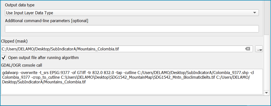
• Click Run to run the tool

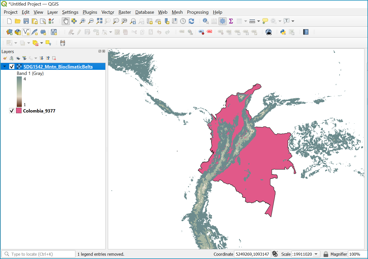
The new clipped mountain descriptor dataset in the national projection should be added to the map canvas.

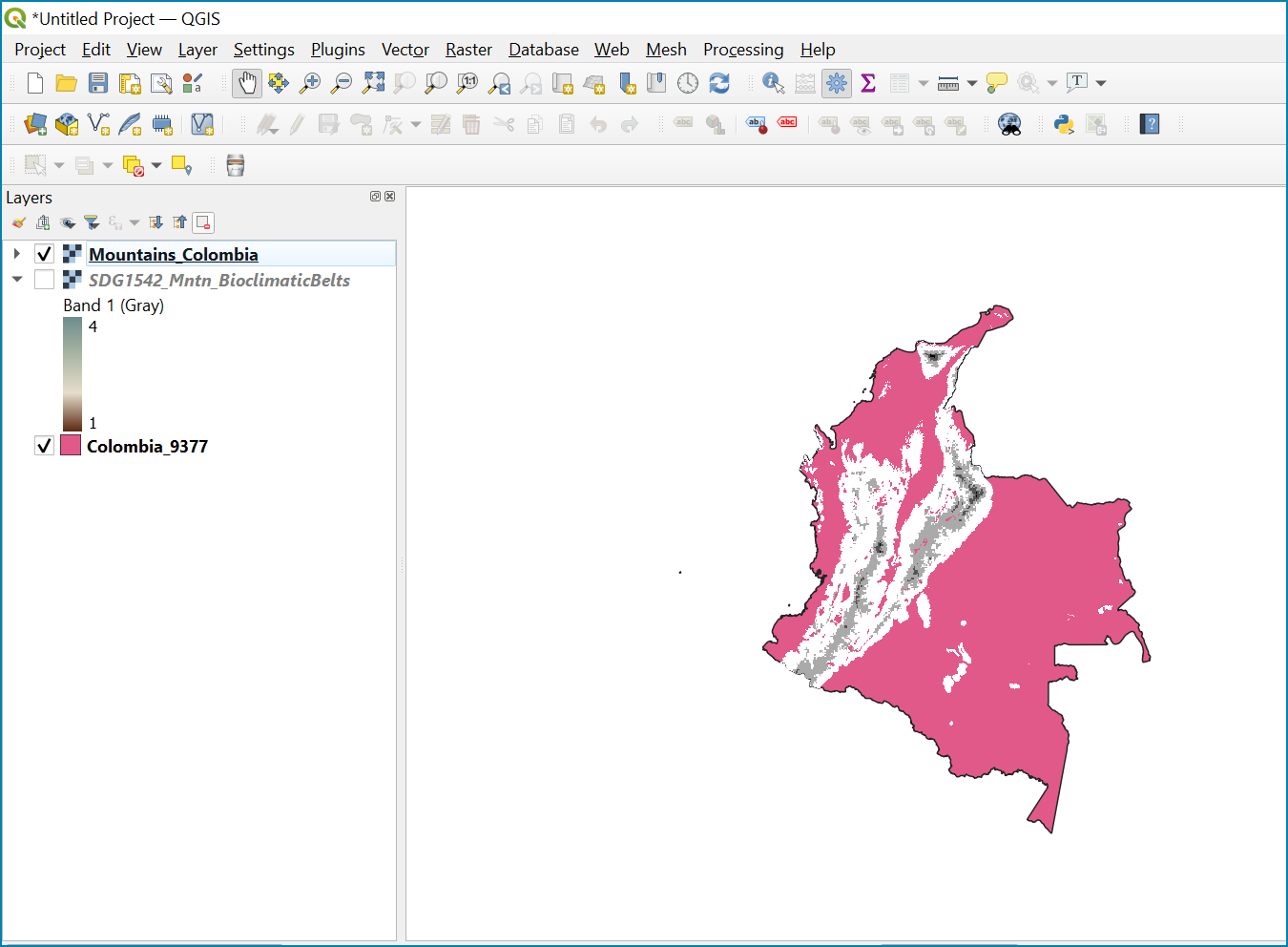
The boundaries and names shown, and the designations used on this map do not imply official endorsement or acceptance by the United Nations.

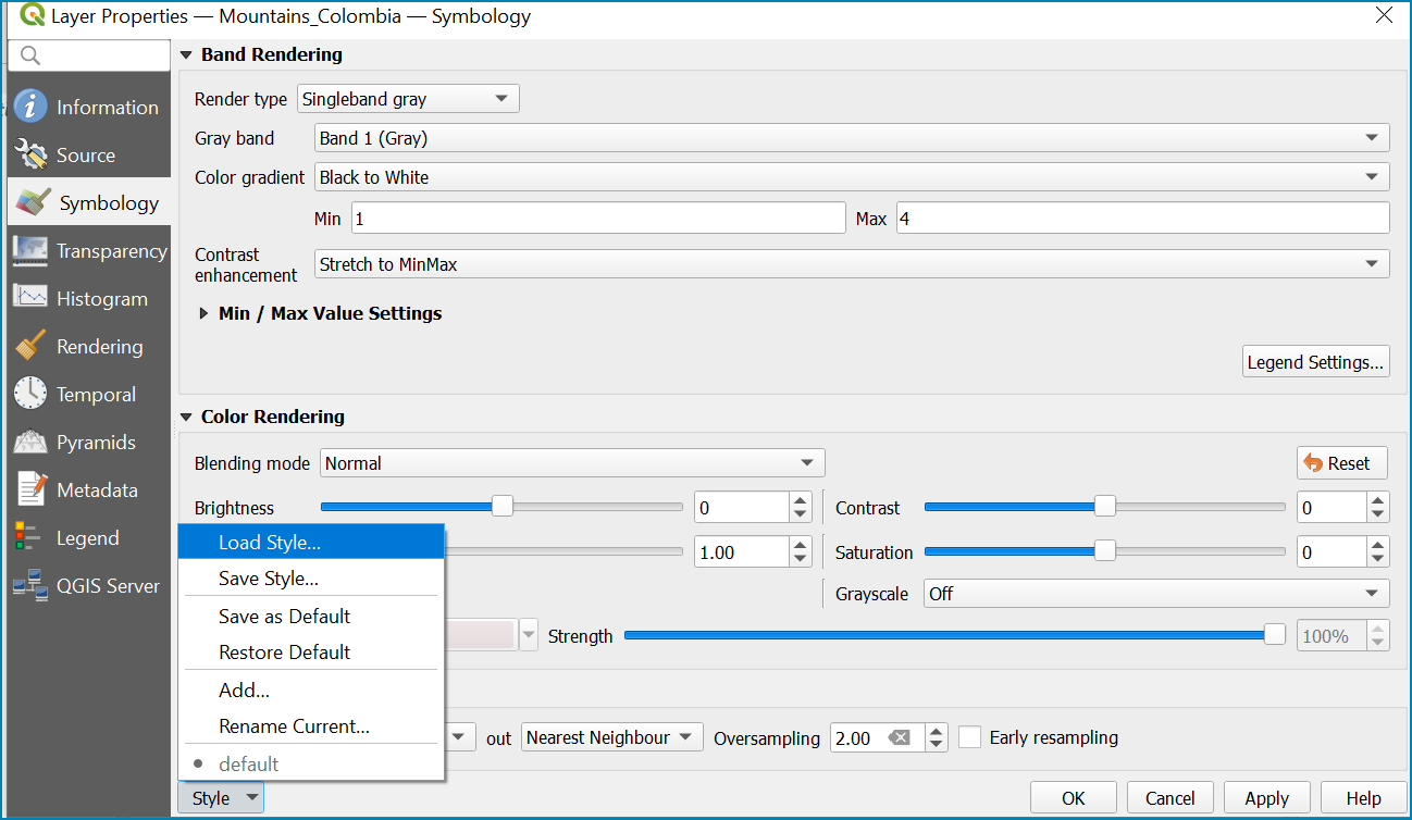
• Right click on the clipped mountain dataset (i.e. in this example the Mountains_Colombia layer) and click properties>>Symbology

• Click on Style >> Load Style, and select the SDG1542_Mntn_BioclimaticBelts.qml included in the Global Descriptor Dataset Folder

The layer should now show all the mountain area for Colombia classified by Biolimatic belts (where 1 is ‘’Nival”, 2 is “Alpine”, 3 is ‘’Montane” and 4 is “Remaining Mountain Area”.

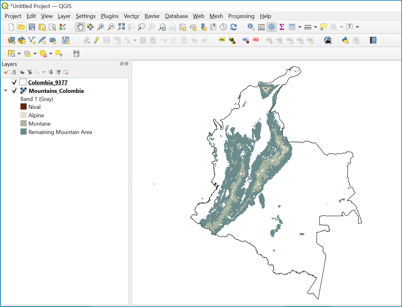
The boundaries and names shown, and the designations used on this map do not imply official endorsement or acceptance by the United Nations.

Combine mountain and vegetation descriptor layers

Now that we have 2 raster datasets in their native resolutions we need to bring the datasets together and ensure that correct aggregation is undertaken and that the all the layers align to a common resolution.

Aggregate the layers to a common spatial resolution

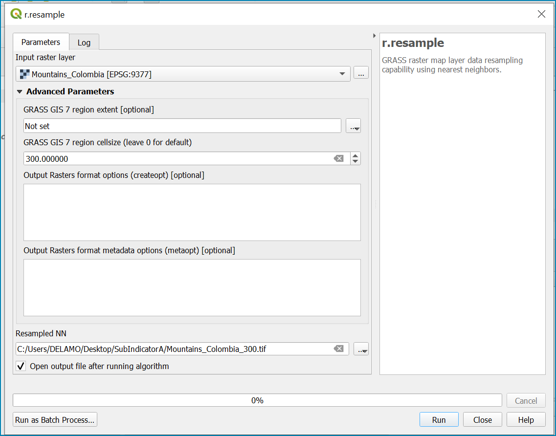
In this example we have the Mountain Descriptor layer at a 832 meters resolution and a vegetation descriptor layer at a 300 m resolution. There are various tools that can be used but we have opted for the GRASS tool r.resample as it allowed to resample the mountain descriptor to the vegetation layer, which has a finer grid.

In the processing toolbox search for *r.resample*

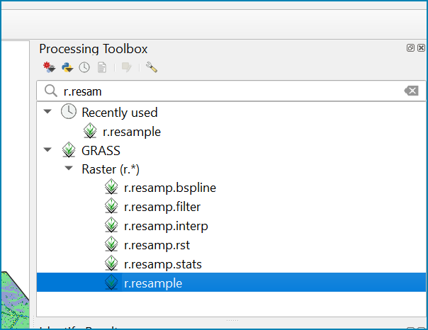
• Select the mountain descriptor (in this example Mountains_Colombia.tif) as the Input Layer

• Set the cellsize to the the same resolution as your Vegetation Descriptor layer e.g. in this example 300m

• Set the Resampled Aggregated layer to a name that distinguishes the resampling of the layer e.g. Mountains_Colombia_300.tif

• Click Run to run the tool

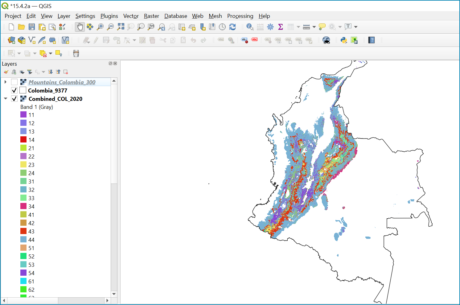
Combine mountain and vegetation descriptor layers

As SGD Indicator 15.4.2a requires disaggregation by both the 10 land cover classes and the 4 bioclimatic belts and the tools within QGIS will only allow a single input for zones, we will combine the two datasets.

• In the processing toolbox, search for and double click on the raster calculator

• In the expression window we will sum the two dataset together but in order to distinguish the vegetation class from the mountain all the vegetation values will be multiplied by 10. This means for example a value of 35 in the output means the pixel has class 3 in the vegetation descriptor layer and class 5 in the Mountain descriptor layer.

• In the expression box formulate the expression:

(“VEGETATION_DESCRIPTOR@1”* 10) + “MoutainDescriptor@1”

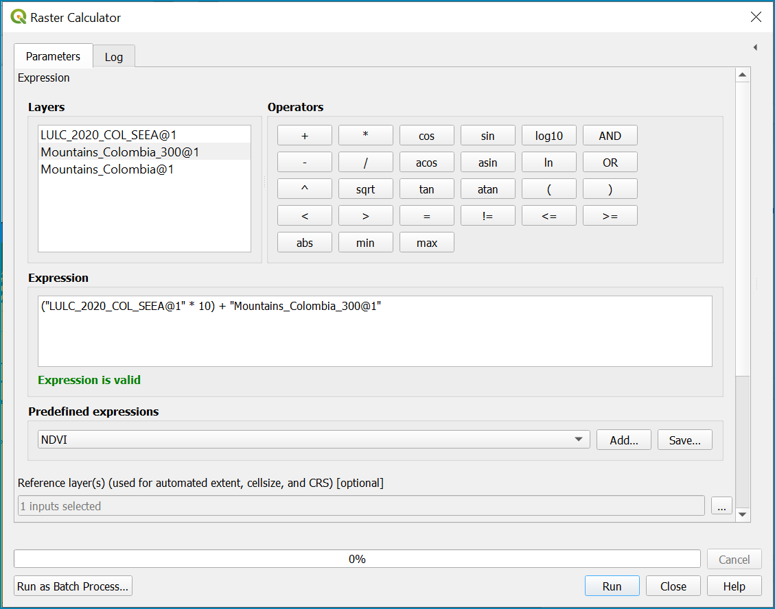
• Set the Reference layer as the Vegetation Descriptor layer

• Click Run to run the tool

The boundaries and names shown, and the designations used on this map do not imply official endorsement or acceptance by the United Nations.

Step-by-step equivalent of Tool step A3 download DEM

The step guides users in downloading an appropriate DEM. Please refer to the Defining environments section and Annex 1 for more information download options. If you are not calculating Real Surface Area, this step will not be required.

Step-by-step equivalent of Tool step A4 Generate real surface area raster

This step cannot be carried out manually. Please run the QGIS model Step A4 which runs an R script to calculate Real Surface Area.

Computation of Sub-indicator a Mountain Green Cover Index

Step-by-step equivalent of Tool Step A5 Generate planimetric and real surface area statistics

The following steps are covered by this tool:

NOTE: the step by step instructions only calculate planimetric area. For real Surface Area statistics the toolbox must be used.

Generate area statistics for each land cover class

The data are now in a consistent format, so we can now generate the statistics required for the MGCI reporting. As we want to generate disaggregated statistics by LULC class and bioclimatic belt we will use a zonal statistics tool with the combined Vegetation + mountain layer as the summary unit. The Zonal statistics tool will automatically calculate planimetric area in the output.

This output is the main statistics table from the analysis, from which other summary statistics tables will be generated.

• In the processing toolbox search for Zonal Statistics

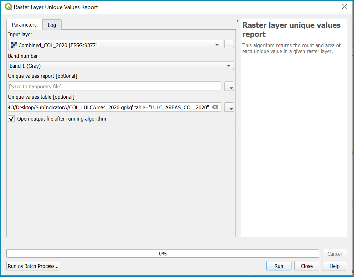
• Double click on the Raster layer unique values report.

• Set the input layer to the combined vegetation and mountain class layer created in the previous step.

• Under the Unique values table click on … and choose Save to File…. Enter a name for the file, in this case LULC_Areas_COL_2020.gpkg.

• Click Run.

Now the LULC_Areas_COL_2020  layer will be added to the Layers panel. Right-click on the layer and click Open Attribute Table. The column m2 contains the area for each class in square meters.

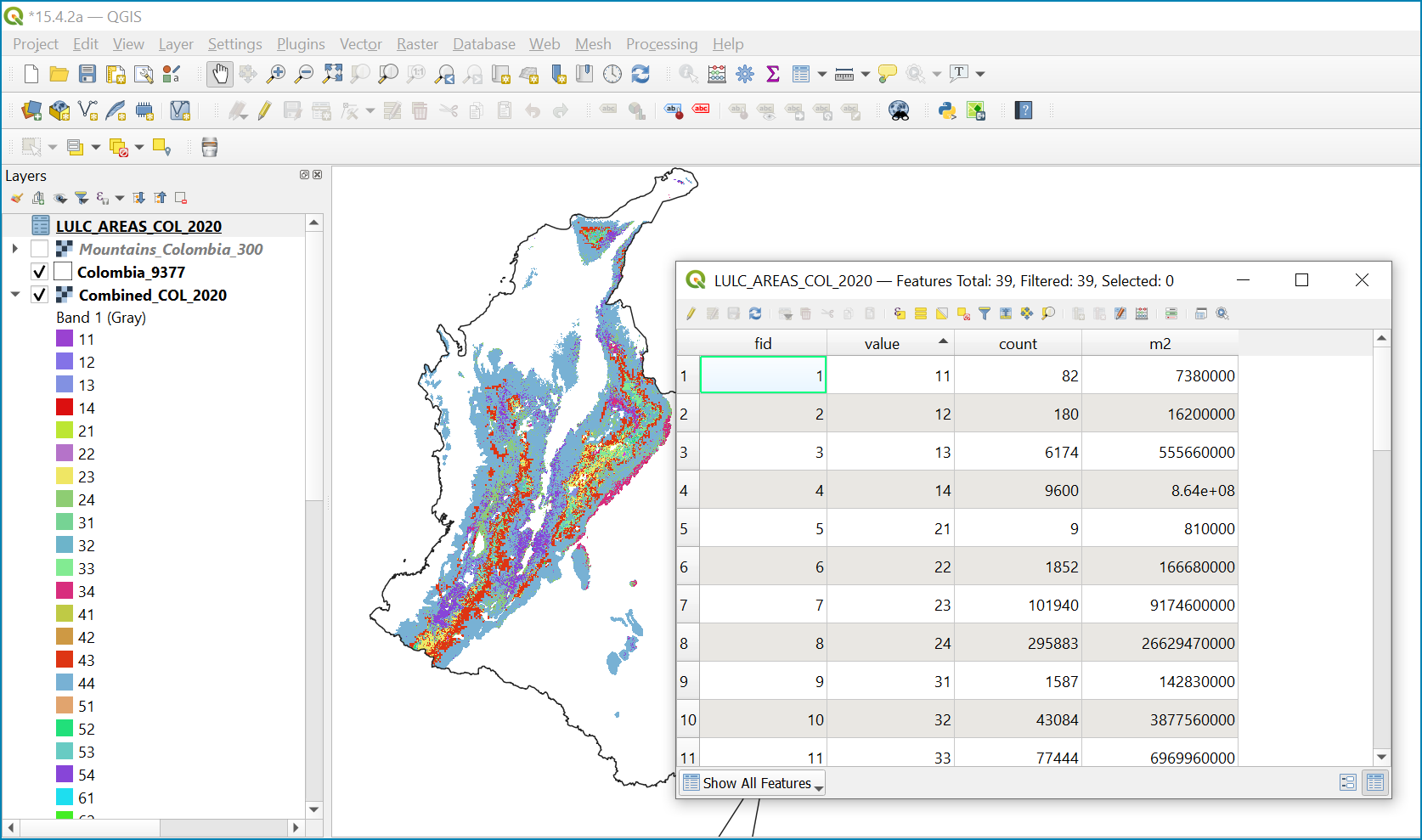
The boundaries and names shown, and the designations used on this map do not imply official endorsement or acceptance by the United Nations.

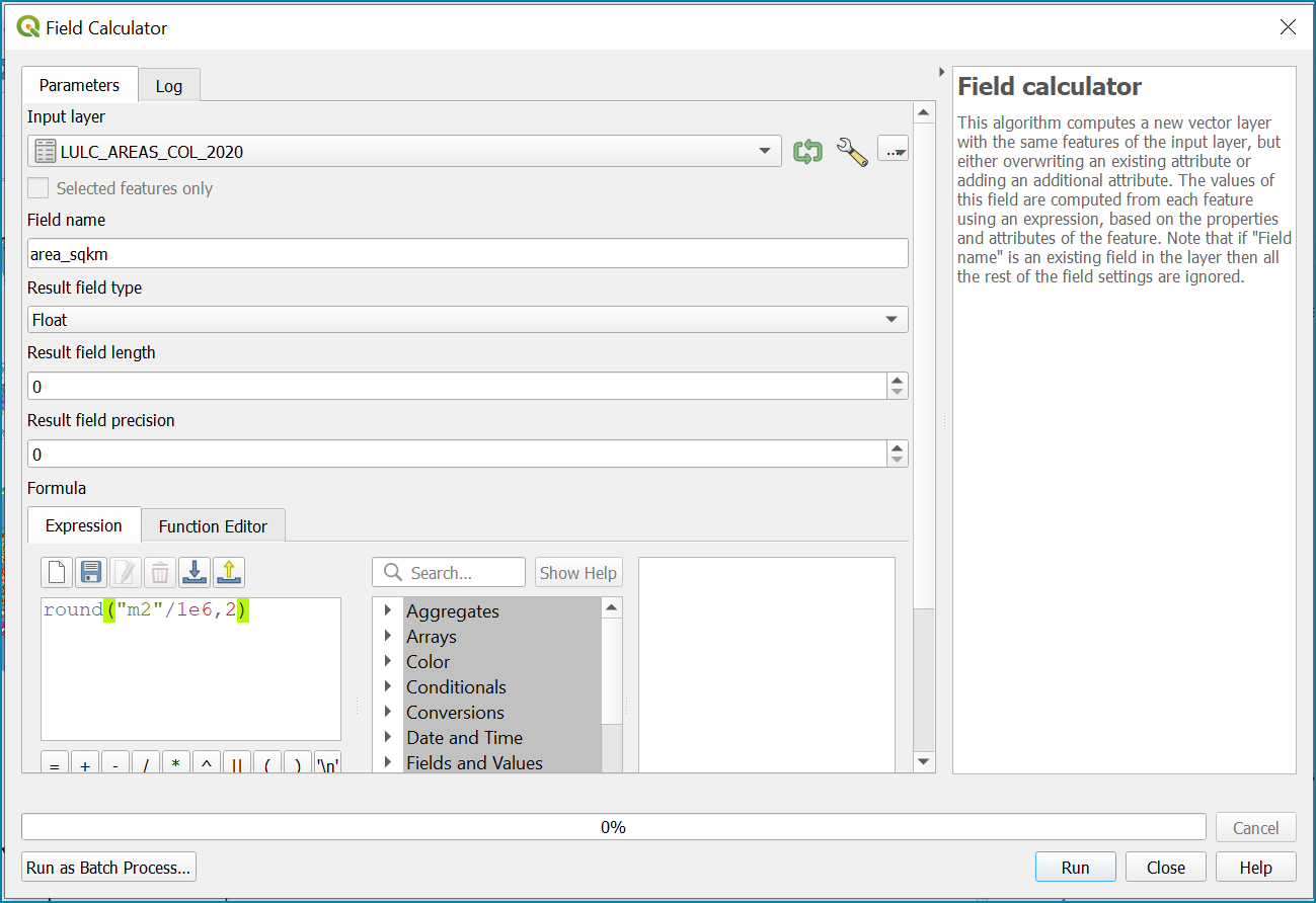
Let’s convert the area to square kilometers. In the Processing Toolbox, search and select Vector table >> Field Calculator.

• In the Field Calculator dialog, select the LULC_Areas_COL_2020 layer

• Enter the Field name as Area_sqkm.

• In the Result field type choose Float

• In the Expression window, enter the below expression. This will convert the sqmt to sqkm and round the result to 2 decimal places. Under the Calculated click on … and choose Save To File… . Enter the name as LULC_Areas_COL_2020_sqkm.csv

  round(“m2”/1e6, 2)

• Click Run.

Now the LULC_Areas_COL_2020_sqkm will be loaded in canvas. Open the Attribute table and examine the newly added area_sqkm column. You will notice that the Value column contains numbers for each class. To make the results easier to interpret. Let’s also add the land cover name for each class number

In the Attribute Table, select “ Open Field Calculator” in the top bar.

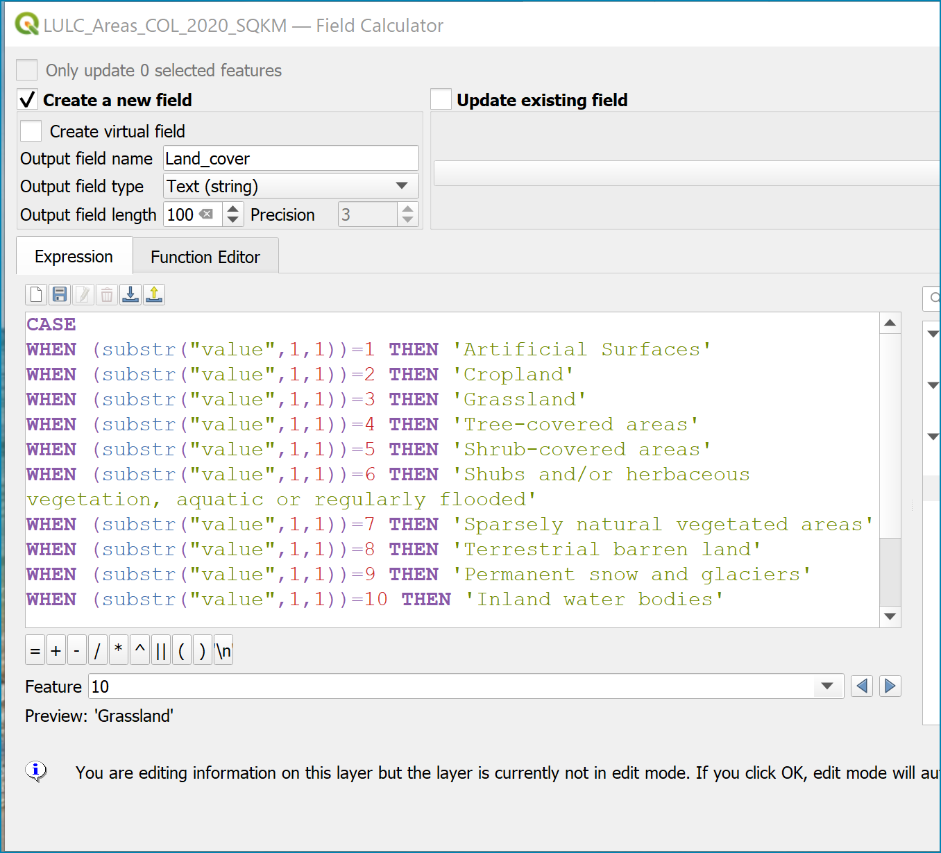
• Enter the Field name as Land_cover.

• In the Result field type, choose String. In Output field length enter 100.

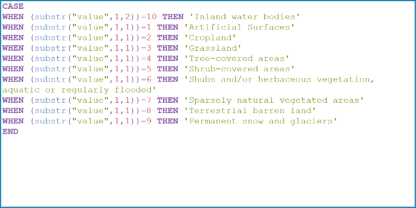
• In the Expression window enter the below expression. This expression uses the CASE statement to assign a value based on multiple conditions. In this case it extract the first string of the value field, which indicate the type of land cover, to assign the name of the land cover in the new field name called “Land cover”

CASE

WHEN (substr(“value”,1,2))=10 THEN ‘Inland water bodies’

WHEN (substr(“value”,1,1))=1 THEN ‘Artificial Surfaces’

WHEN (substr(“value”,1,1))=2 THEN ‘Cropland’

WHEN (substr(“value”,1,1))=3 THEN ‘Grassland’

WHEN (substr(“value”,1,1))=4 THEN ‘Tree-covered areas’

WHEN (substr(“value”,1,1))=5 THEN ‘Shrub-covered areas’

WHEN (substr(“value”,1,1))=6 THEN ‘Shrubs and/or herbaceous vegetation, aquatic or regularly flooded’

WHEN (substr(“value”,1,1))=7 THEN ‘Sparsely natural vegetated areas’

WHEN (substr(“value”,1,1))=8 THEN ‘Terrestrial barren land’

WHEN (substr(“value”,1,1))=9 THEN ‘Permanent snow and glaciers’

END

• Click Run.

Do the same again to add the Bioclimatic belt for each end string for each value number, using the below expression:

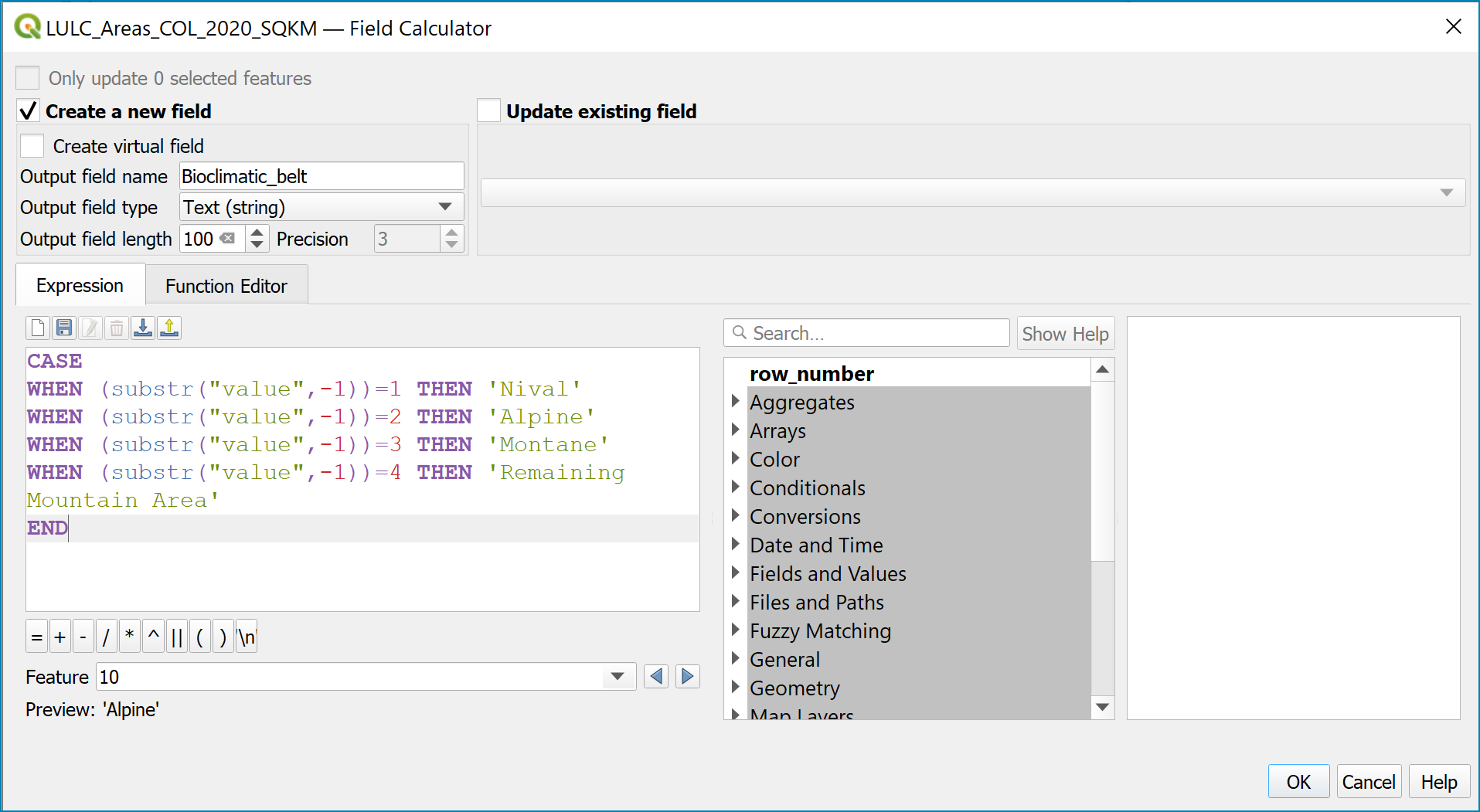
CASE

WHEN (substr(“value”,2,1))=1 THEN ‘Nival’

WHEN (substr(“value”,2,1))=2 THEN ‘Alpine’

WHEN (substr(“value”,2,1))=3 THEN ‘Montane’

WHEN (substr(“value”,2,1))=4 THEN ‘Remaining Mountain Area’

WHEN (substr(“value”,3,1))=1 THEN ‘Nival’

WHEN (substr(“value”,3,1))=2 THEN ‘Alpine’

WHEN (substr(“value”,3,1))=3 THEN ‘Montane’

WHEN (substr(“value”,3,1))=4 THEN ‘Remaining Mountain Area’

END

Save the edits.

Step-by-step equivalent of Tool Step A6 Formatting to reporting tables

The following steps are covered by this tool (although when undertaken manually the steps are slightly different as a QGIS plugin can be used to help with the formatting):

Now, we will export this result as an excel file. Before export we will also organize the table and remove unwanted fields. In the Processing Toolbox, search and select Vector table ‣ Refactor fields.

In the Refactor Fields dialog, select the layer edited in the prior step as an Input layer (in this case LULC_Areas_COL_2020_SQKM), select all columns except area_sqkm, Land_cover, Bioclimatic_belt and then click Delete selected field.

Once you are done with the edits, click on the … button next to Refactored and choose Save To File…. Select XLSX Files (*.xlsx) as the format. Enter the file name as 15.4.2a_2020.xlsx and click Save. In the Refactor Fields dialog, click Run to apply your changes.

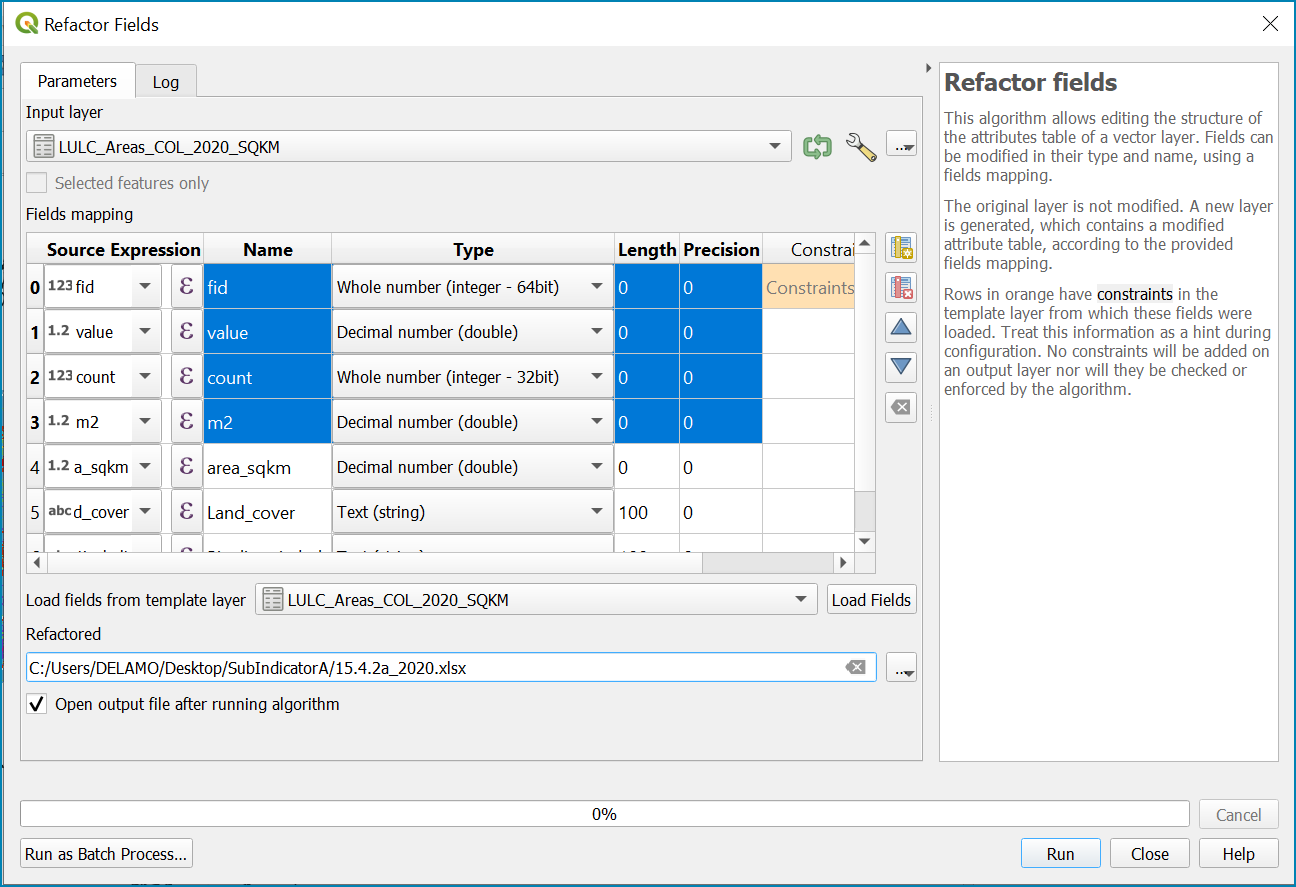
The result will be a spreadheet with area_sqkm , land_cover and Bioclimatic_belt columns.

In Excel, calculate: (1) the total area of each bioclimatic belt (by summing the area of all land cover types per bioclimatic belt); (2) the total area of each land cover type across all bioclimatic belts (by summing the area of each specific land cover type across all bioclimatic belts) and finally; (3) the total mountain area of the country (by summing the area of all land cover types across all bioclimatic belts).

Save this excel tab as 15.4.2a_dis_landcover. This data contains the estimates of 15.4.2 sub-indicator a, disaggregated by land cover type. Let’s now calculate the Mountain Green Cover Index estimates.

Copy and paste the values of this tab into another tab. In this one, calculate Green Cover area for each bioclimatic belt, by summing the areas of the following land cover types: (1) Tree-covered areas, (2) Grasslands, (3) Croplands, (4) Shrub-covered areas and (5) Shubs and/or herbaceous vegetation, aquatic or regularly flooded.

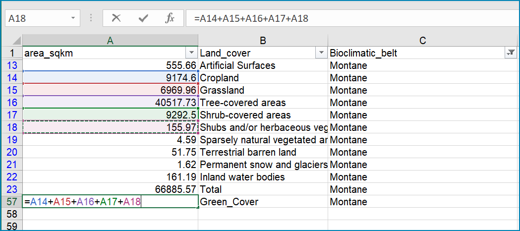
Finally, calculate the MGCI by diving the area of green cover the total area of each bioclimatic belt and the total mountain area and multiplying it by 100.

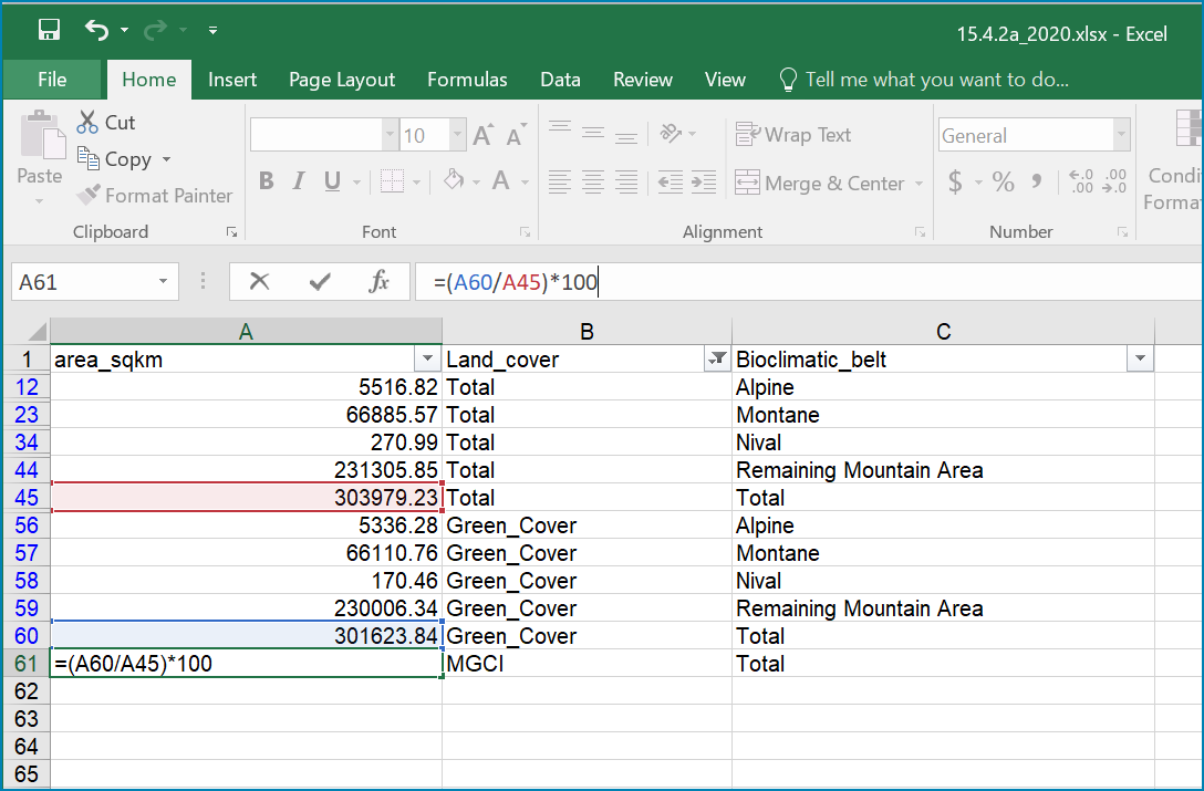
Sub-indicator a is now complete.

Repeat for each of the reporting years.

Manual steps to calculate Sub-indicator 15.4.2b in QGIS

This section of the tutorial explains in detail how to calculate value estimates for sub-indicator 15.4.2b in QGIS, continuing to use Colombia as a case study. Sub-Indicator 15.4.2b is designed to monitor the extent of degraded mountain land as a result of land cover change of a given country and for given reporting year.

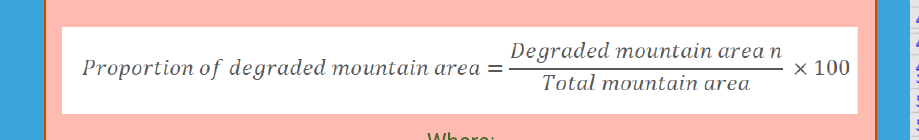
This sub-indicator looks at the proportion of degraded mountain area, calculated using a binary score (degraded/non-degraded) showing the extent of degraded land over total mountain area. This is calculated using the following formula:

Where:
Degraded mountain area *n* = Total degraded mountain area (in Km2) in the reporting period n. This is, the sum of the areas where land cover change is considered to constitute degradation from the baseline period.
Total mountain area = Total area of mountains (in Km2).

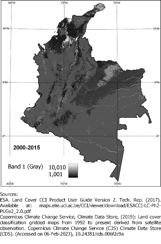
As a reminder, in accordance with the SDG indicator’s metadata countries are required to compute estimates for Sub-Indicator 15.4.2b for a baseline for approximately 2000-2015, and subsequently every three years (2018, 2021, 2024, 2027 and 2030). Therefore, for the example in this tutorial we will use the ESA-CCI landcover products for 2000, 2015 (for the baseline) and 2018 (for the reporting year). ESA-CCI landcover data are not yet available beyond 2021 so we have therefore not yet been able to calculate subsequent years in this example.

This section of the tutorial assumes that the user has already calculated sub-indicator 15.4.2a and has therefore already downloaded and translated the landcover cover datasets to UN-SEEA classes for the baseline and reporting years (see sections 3.1-3.3 of the tutorial) as presented in the figure below).

LULC reclassified into UN-SEEA classes for 2000, 2015 and 2018

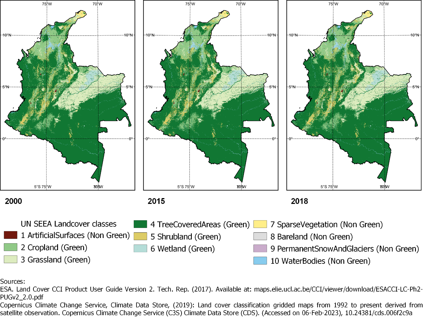
The boundaries and names shown, and the designations used on this map do not imply official endorsement or acceptance by the United Nations.

SGD Indicator 15.4.2b requires us to identify change between LC classes in each reporting period, therefore the first requirement for sub-indicator 15.4.2b is to develop a transition matrix that specifies the land cover changes occurring in a given land unit (pixel) as being either degradation, improvement or neutral transitions. The definition of degradation adopted for the computation of this indicator is the one established by the Intergovernmental Science-Policy Platform on Biodiversity and Ecosystem Services (IPBES) [2].

Countries may choose to either calculate degradation using the default land cover legend for this indicator and default transition matrix provided or from a native or simplified legend of a national land use/land cover (LULC) dataset if they have the advantage of better representing degradation transitions compared to the broader default transitions.

Section 4.1.1 describes the default method using the default legend and transition matrix, while section 4.1.2 outlines the additional/alternative steps required to generate a transitions matrix using a nationally adapted land cover legend. In both cases the output results in the same 3 classes (stable, degradation and improving) and both needed to be disaggregated and reported by both landcover transition and bioclimatic belt.

The easiest method in QGIS is to generate a single value that represents both year1 landcover and year2 landcover. For example, when calculating the baseline using the default land cover legend reclassified datasets for 2000 and 2015, each dataset has LULC values from 1-10 we need to change the values for one of the years to be able to distinguish between classes in year1 and year2. When using the nationally adapted LULC legend, the values may be greater than 1-10. We will therefore multiply values in year 1 by 1000 (in order to avoid any overlap between the values in year 2).

Step-by-step equivalent of Tool Step B1 Combine LULC datasets

The following steps are covered by this tool:

Combine the landcover dataset for the baseline and reporting year

First, we will generate a single raster containing a value to represent both year1 landcover and year2 landcover. We will demonstrate using the default method using the UN-SEEA reclassified landcover raster’s in equal area projection that were previously reclassified for the computation of sub-indicator a. As indicated above, users can choose to use the rasters projected to equal area projection containing the full or a simplified national LULC legend if there is a preference/advantage of calculating landcover transitions compared to using the default legend and transition matrix. The processing is the same regardless which method is chosen.

In this example we will use the UN-SEEA reclassified landcover datasets for 2000 and 2015 for the baseline and UN-SEEA classified landcover 2015 to 2018 raster’s for the 2018 reporting year. As each dataset has the same LULC values (values 1-10 for UN-SEEA classification) we need to change the values in one of the years to be able to distinguish between classes in year1 and year2. We will multiply year1 land cover classes by 1000 before summing the datasets together. So for example values for year 1 when using the default legend will range from 1000 – 10000 and values for year 2 will remain 1 -10 and the resultant output will have values ranging from a minimum of 1001 to a maximum of 10010 (depending on which LULC transitions are present).

We will calculate the baseline period first i.e. using 2000 landcover (year 1) and 2015 landcover (year2)

• In the processing toolbox, search for and double click on the raster calculator

• In the expression box formulate the expression (in this example using the UN-SEEA datasets):

(“UNSEEA_LULC2000_BND_AOI_EqArea@1”* 1000) + “UNSEEA_LULC2015_BND_AOI_EqArea@1”

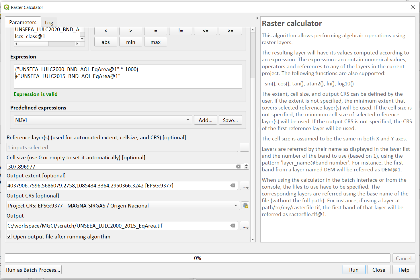
The boundaries and names shown, and the designations used on this map do not imply official endorsement or acceptance by the United Nations.

Set the Reference layer as one of the landcover datasets

to set the extent, cellsize and CRS e.g. UNSEEA_LULC2015_BND_AOI_EqArea layer

• Set the Output dataset to a new name e.g. UNSEEA_LULC2000_2015_BND_AOI_EqArea.tif for the baseline

• Click Run to run the tool

When using the default UN-SEEA land cover legend, this means that a value of 2001 means a land cover class 2 in year 1 and a land cover class 1 in year 2. A value of 10010 would mean a land cover class 10 in year 1 and a land cover class 10 in year 2. In other words, year 1 is represented by the first digit for values 1 to 9, and by the first 2 digits for land cover class 10. Year 2, on the other hand, is represented by the right hand digit (for values 1-9) and the right hand 2 digits for value 10.

Repeat the above step for the next reporting period i.e. using 2015 landcover (year 1) and 2018 landcover (year2)

Step-by-step equivalent of Tool Step B2 Generate Transition matrix

The following steps are covered by this tool:

Generate the transitions Matrix

Option 1: Use the default transitions matrix (using the default LULC legend)

Download the default transitions matrix csv file from the GitHub repository showing the unique combination of transitions using the default UN-SEEA classes as presented in the figure below. The default transitions matrix lists the transitions from the LULC classes to the 3 change classes Stable (0), Degradation (-1) and Improving (1).

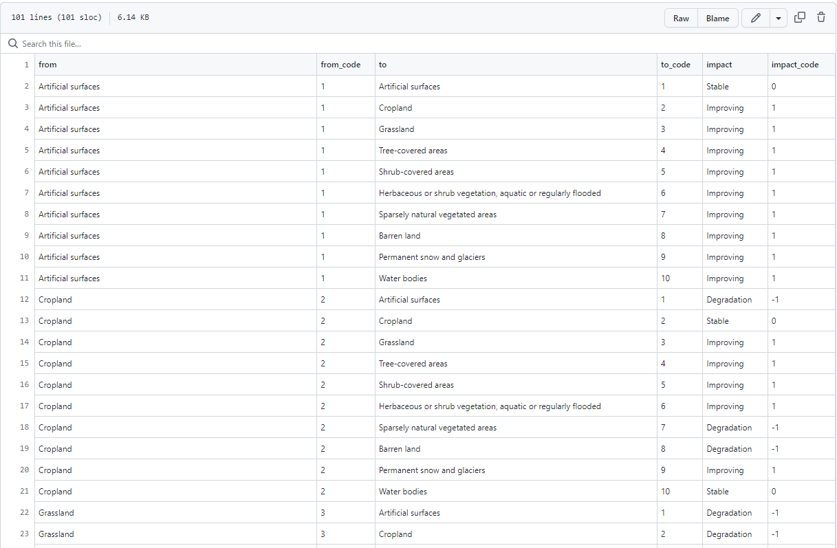
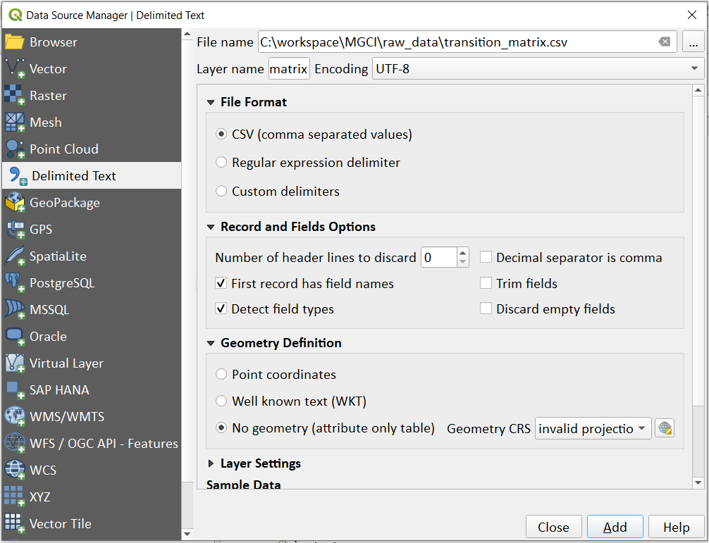
• Download the transitions matrix csv file and add it to your QGIS project using Layer>>Add Layer>>Add Delimited Text Layer

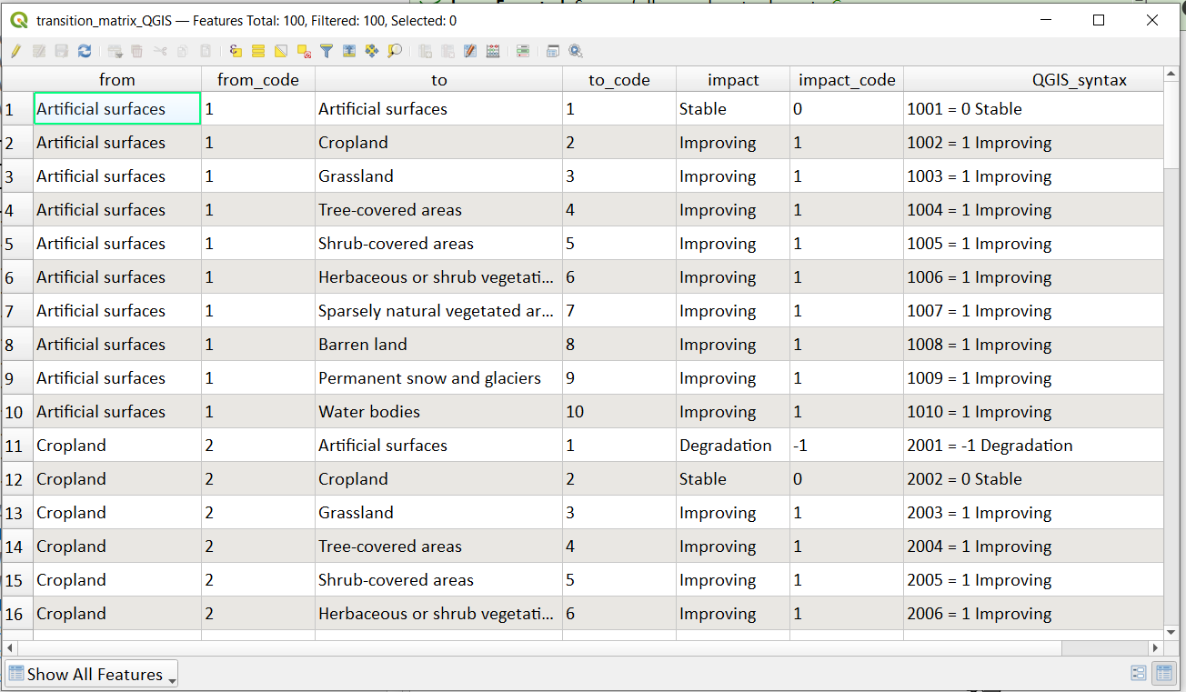
Despite the clarity of this format transitions matrix, the reclassification tools in QGIS require a very specific format for the reclassification table. We therefore need to add an additional field and calculate it to be the required QGIS syntax. This field will then be saved into a new CSV file which can be used by the QGIS geoprocessing tool.

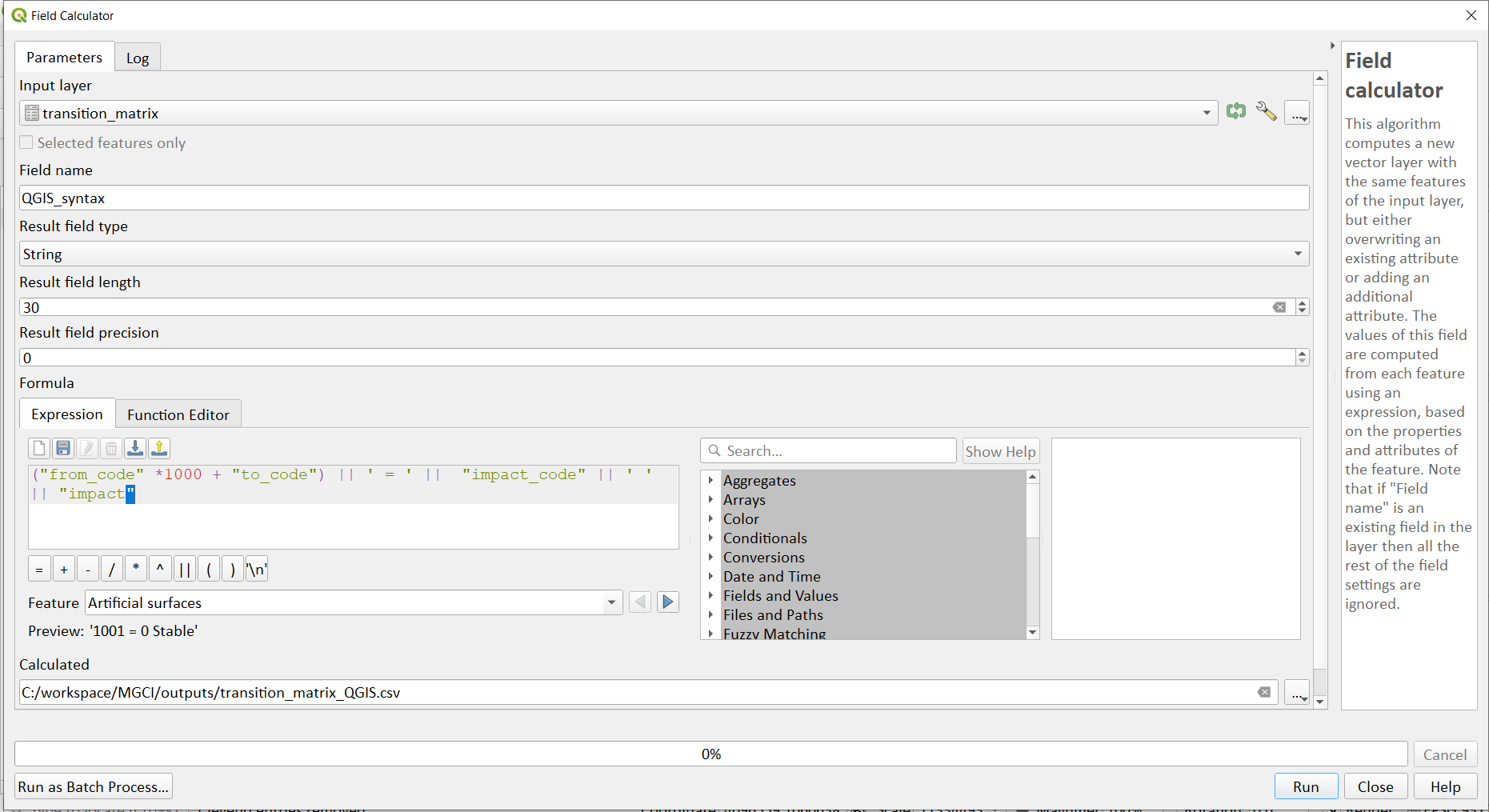
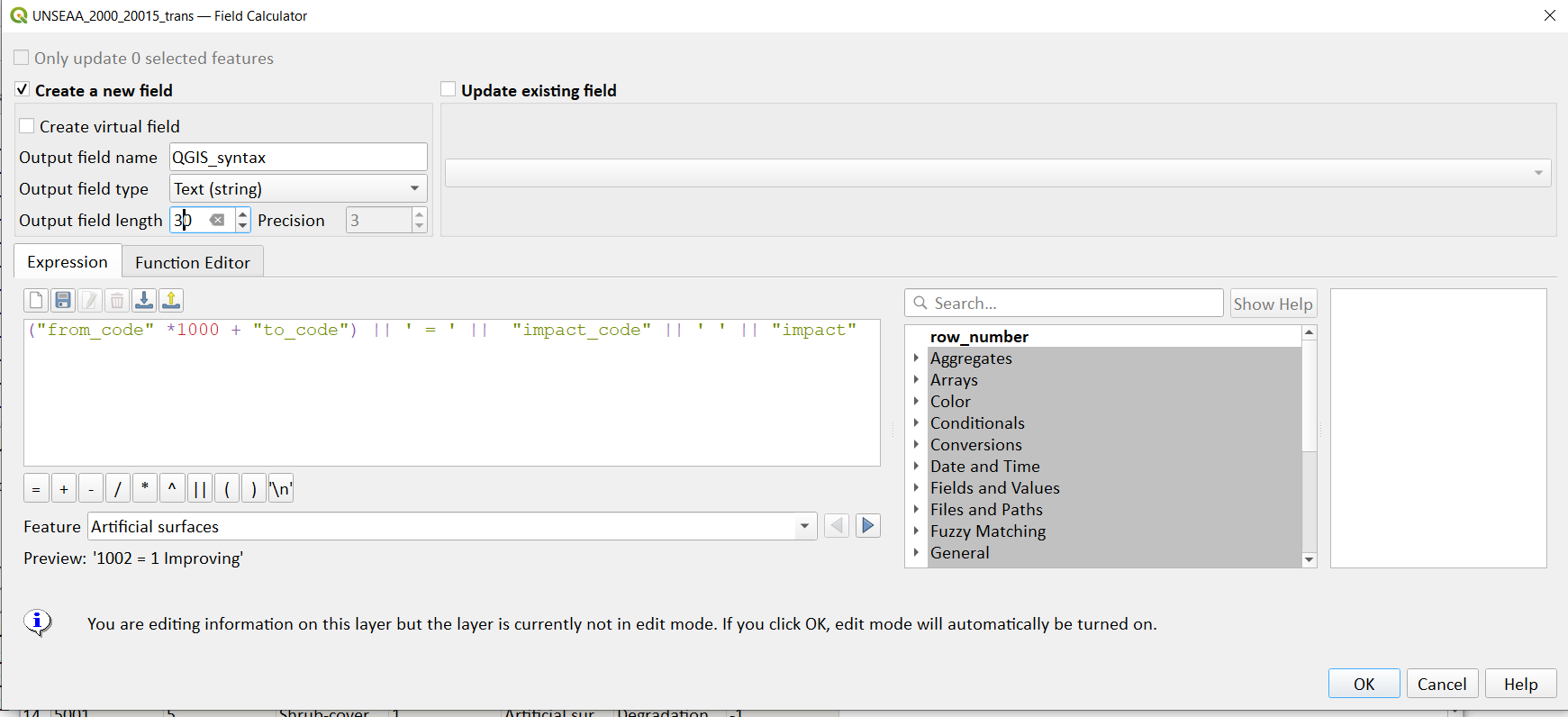
• In the Geoprocessing toolbox search for Field Calculator

In the field calculator add a new string field called QGIS_syntax with length 30.

In the expression builder paste in the following text. Note that we are taking the Landcover code for year 1 and multiplying it by 1000 (as described above) and summing it with the landcover code for year 2 before combining it with the rest of the QGIS syntax

(“from_code” *1000 + “to_code”) || ‘ = ‘ || “impact_code” || ‘ ‘ || “impact”

The resultant table should look like this:

• Next search for the List unique values tool in the geoprocessing toolbox, this will be used to export the new column, QGIS_syntax to a new csv file

• Select the transitions_matrix_QGIS as the input layer

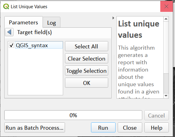
Select the QGIS_syntax field in the target field

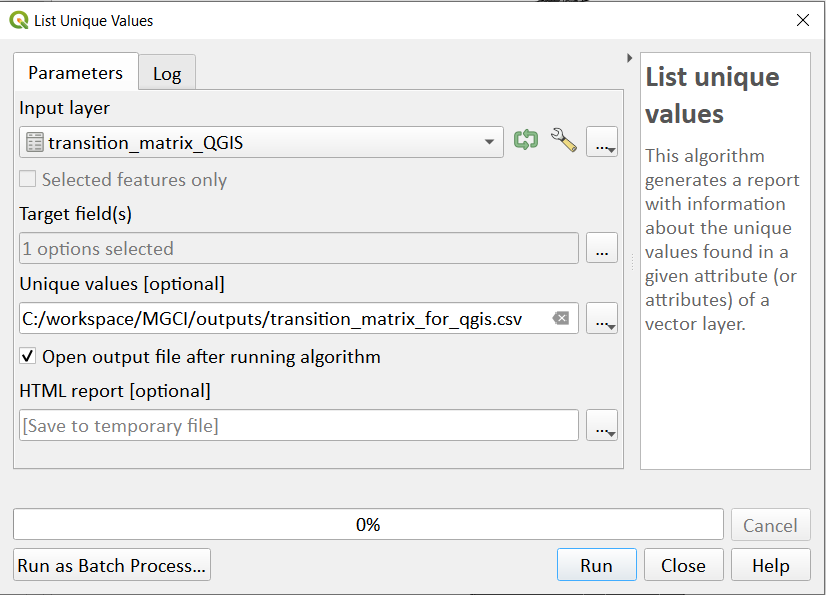
• Save the unique values to a new csv file e.g. transition_matrix_for_qgis.csv

• Click Run

• Outside QGIS, open a windows explorer window navigate to the csv file and open in notepad

• Remove the header row and save the file as transition_matrix_for_qgis.txt

• Return to QGIS

Option 2: Generate a transitions matrix using a national LULC

If are using a national land cover transition matrix you can prepare a transitions table in the same format as the default transitions table in Excel or you can generate a csv file from the unique combinations for the LULC types using the combined LULC dataset for the two years. We illustrate this below (although we are using the default UN-SEEA classes for illustration purposes only)

• In the processing toolbox search for Raster Layer Unique Values Report

• Select the combined LULC dataset for year 1 and year 2 as the input layer e.g. SEEA_LULC2000_2015_BND_AOI_EqArea.tif

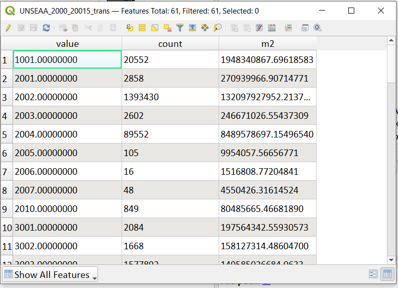
• Set the Unique values report to a new output table e.g. UNSEAA_2000_20015_trans.csv

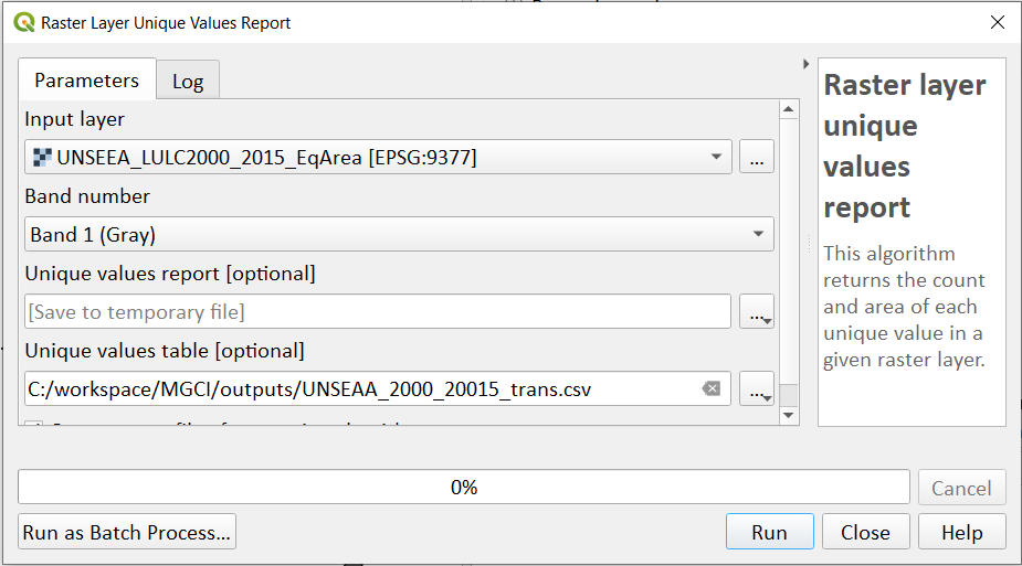
The resultant table looks like this:

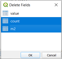
Delete the count and m2 columns by clicking on the toggle editing button on the top menu bar of the attribute table and then click the Delete Field button. Select the “ *count”* and “ *m2* ” fields and click OK to delete

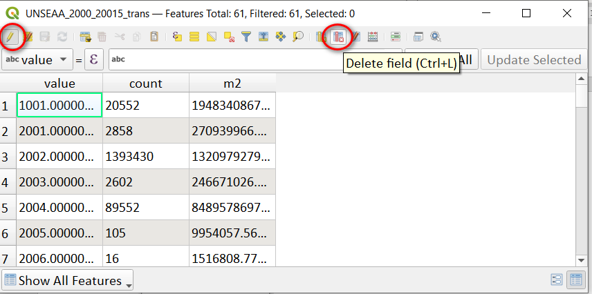
• Click on the toggle editing button on the top menu bar again to save the changes

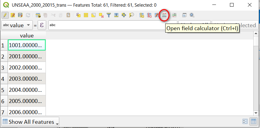
We can then add the to and from codes and descriptions.

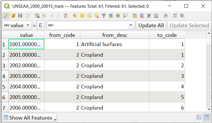
In the Attribute Table, click the “ Open Field Calculator” button in the top bar.

• Enter the Field name as from_code.

• In the Result field type, choose Whole Number (Integer). In Output field length enter 3.

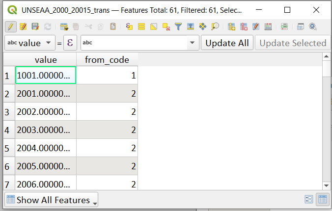
• In the Expression window enter the expression: “value” / 1000

  

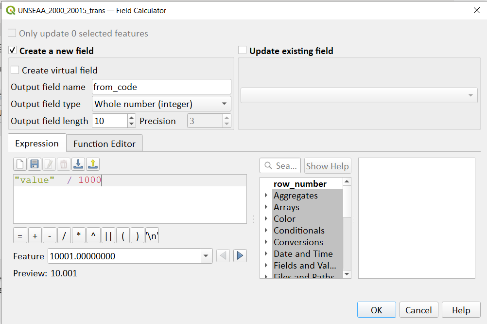
• Click  OK

The result looks like this:

In the Attribute Table, select “Open Field Calculator” in the top bar again.

• Enter the Field name as from_desc.

• In the Result field type, choose Text ( String). In Output field length enter 100.

• In the Expression window enter the below expression, replacing the names of the default UN-SEEEA LULC classes by the names of the national LULC legend. This expression uses the CASE statement to assign a value based on multiple conditions.

  CASE

  WHEN “from_code” =10 THEN ‘Inland water bodies’

  WHEN “from_code” =1 THEN ‘Artificial Surfaces’

  WHEN “from_code” =2 THEN ‘Cropland’

  WHEN “from_code” =3 THEN ‘Grassland’

  WHEN “from_code” =4 THEN ‘Tree-covered areas’

  WHEN “from_code” =5 THEN ‘Shrub-covered areas’

  WHEN “from_code” =6 THEN ‘Shrubs and/or herbaceous vegetation, aquatic or regularly flooded’

  WHEN “from_code” =7 THEN ‘Sparsely natural vegetated areas’

  WHEN “from_code” =8 THEN ‘Terrestrial barren land’

  WHEN “from_code” =9 THEN ‘Permanent snow and glaciers’

  END

  

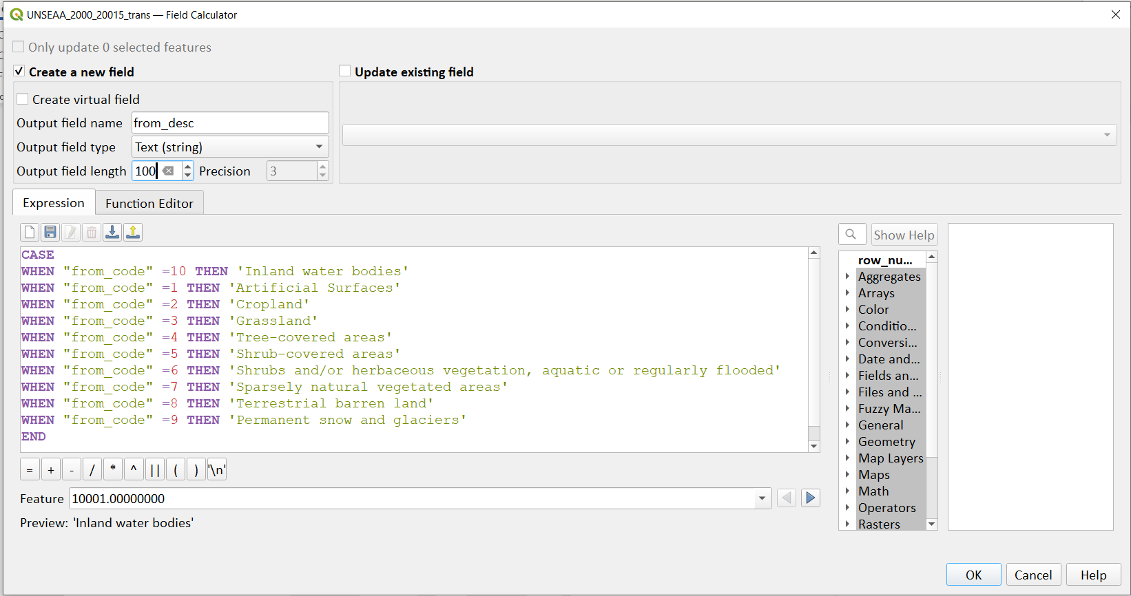
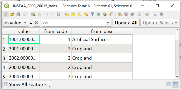
• Click **OK **

  The result looks like this:

  

• In the Geoprocessing toolbox search for Field Calculator

• Enter the Field name as to_code.

• In the Result field type, choose Whole Number (Integer). In Output field length enter 3.

• In the Expression window enter the expression: “value” - (“from_code” *1000)

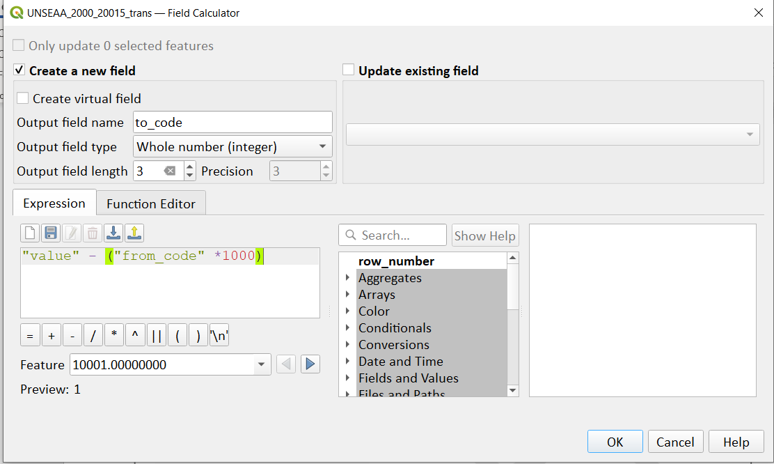
• Click OK

The result looks like this:

In the Attribute Table, select “ Open Field Calculator” in the top bar again.

• Enter the Field name as to_desc.

• In the Result field type, choose Text (String). In Output field length enter 100

• In the Expression window enter the below expression. Again, replacing the names of the default UN-SEEEA LULC classes by the names of the national LULC legend. This expression uses the CASE statement to assign a value based on multiple conditions.

  CASE

  WHEN “to_code” =10 THEN ‘Inland water bodies’

  WHEN “to_code” =1 THEN ‘Artificial Surfaces’

  WHEN “to_code” =2 THEN ‘Cropland’

  WHEN “to_code” =3 THEN ‘Grassland’

  WHEN “to_code” =4 THEN ‘Tree-covered areas’

  WHEN “to_code” =5 THEN ‘Shrub-covered areas’

  WHEN “to_code” =6 THEN ‘Shrubs and/or herbaceous vegetation, aquatic or regularly flooded’

  WHEN “to_code” =7 THEN ‘Sparsely natural vegetated areas’

  WHEN “to_code” =8 THEN ‘Terrestrial barren land’

  WHEN “from_code” =9 THEN ‘Permanent snow and glaciers’

  END

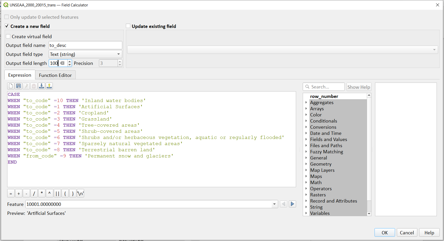
• Click OK.

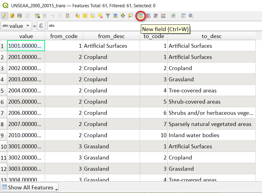
• The result looks like this

• Next click the New Field button to add the following 2 fields

  

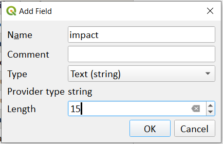
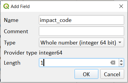
Users can then either manually enter the impact (stable, degradation or improving) and impact_codes (0,-1,1) or use the select button to select groups of transitions and calculate to particular impact types

e.g. select those landcover types that have not changed between year 1 and year 2 and calculate as impact code = 0 and impact = “stable”

• Click on the Select features using and expression button

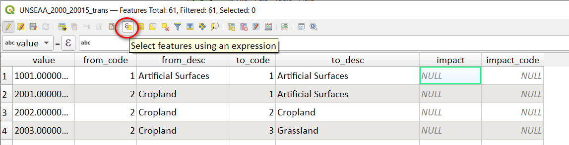
• In the expression box enter the expression “from_code” = “to_code”

• Click Select features

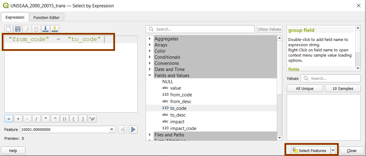
The selected features are highlighted in blue:

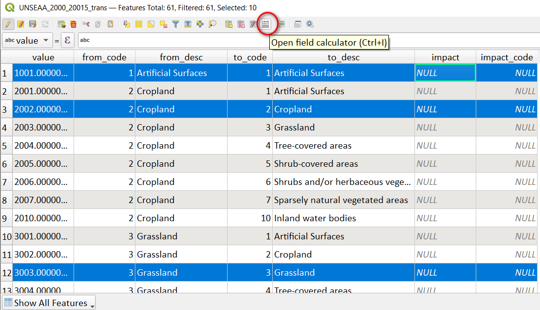
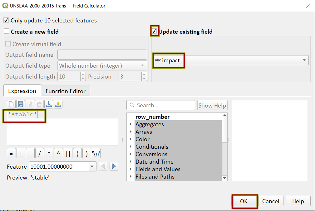
• Click on the Open field calculator button

• Tick Update existing field

• Choose the impact field

• In the expression box type ‘stable’

• Click OK

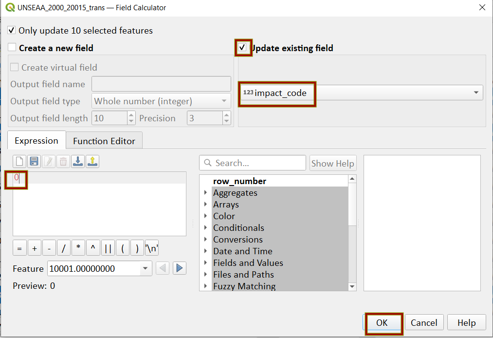• Click on the Open field calculator button again

• Tick Update existing field

• Choose the field impact_code

• In the expression box type 0

• Click OK

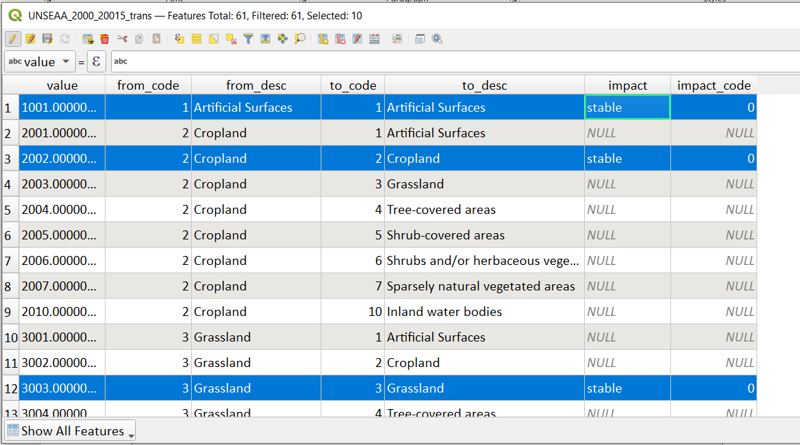
The selected features highlighted in blue are now populated:

Once all the impact values are populated, we need to add an additional field as the reclassification tools in QGIS that will use the transitions matrix require a very specific format for the reclassification table. This field will then be saved into a new CSV file which can be used by the QGIS geoprocessing tool.

• Click on the Open field calculator button

  In the field calculator add a new string field called QGIS_syntax with length 30.

  In the expression window paste in the following text. Note that we are taking the Landcover code for year 1 and multiplying it by 1000 (as described above) and summing it with the landcover code for year 2 before combining it with the rest of the QGIS syntax:

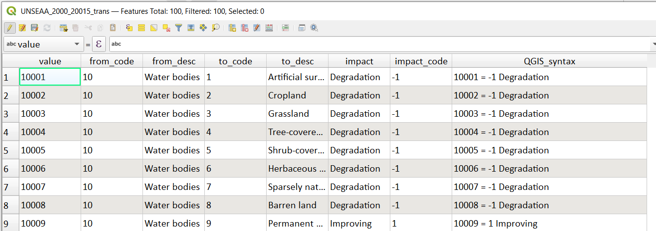
  (“from_code” *1000 + “to_code”) || ‘ = ‘ || “impact_code” || ‘ ‘ || “impact”

  

• Click OK

The resultant table should look like this:

• Next search for the List unique values tool in the geoprocessing toolbox, this will be used to export the new column, QGIS_syntax to a new csv file

• Select the UNSEA_2000_2015_trans as the input layer

• Select the QGIS_synta x field in the target field

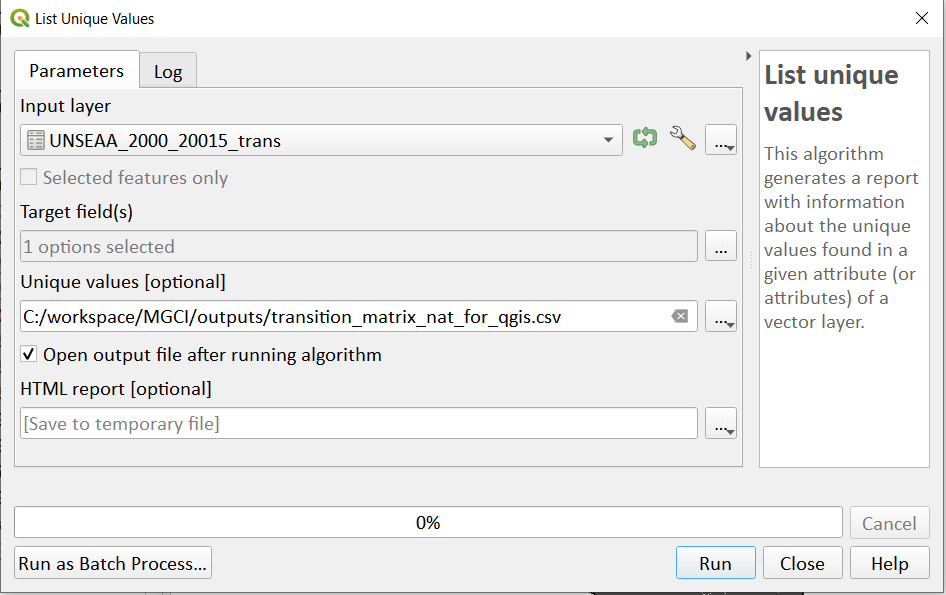
• Save the unique values to a new csv file e.g. transition_matrix_nat_for_qgis.csv

• Click Run

*Important* *Note: Be careful if using this same table for other time periods as it is based on transitions between two specified time periods. E.g. in this case 2000 and 2015. There may be other possible transitions that are not present in this time period but may be possible for other years. Therefore, before using this transitions matrix for other time periods either check for missing entries and manually add them to this table or generate a new transitions table for the new time period.*

Step-by-step equivalent of Tool B3 Reclassify LULC transitions to impact

The following steps are covered by this tool:

Reclassify LULC transitions using the transitions matrix

The next step is to reclassify the outputs from step 5.2 (i.e. the combined landcover datasets for year1 and year 2), first for the baseline period UNSEEA_LULC2000_2015_EqArea.tif and then for the 2018 reporting period UNSEEA_LULC2015_2018_EqArea.tif. We will use the transitions matrix generated in the previous steps (5.3.1 or 5.3.2). In this example we use the default transitions matrix (from 5.3.1) but the steps are the same if a national transitions matrix is being used.

• In the processing toolbox search for r.reclass

• Set the input raster layer to UNSEEA_LULC2000_2015_EqArea.tif

• Set the file containing the reclass rules by navigating to the transitions matrix e.g. transition_matrix_for_qgis.csv

• Set the GRASS GIS 7 Region extent to UNSEEA_LULC2000_2015_EqArea.tif

• Set the cellsize to be the same as UNSEEA_LULC2000_2015_EqArea.tif e.g. in this case 307.896977

• Save the reclassified file to a new name e.g. UNSEEA_LULC2000_2015_EqArea_reclassed_impact.tif

  

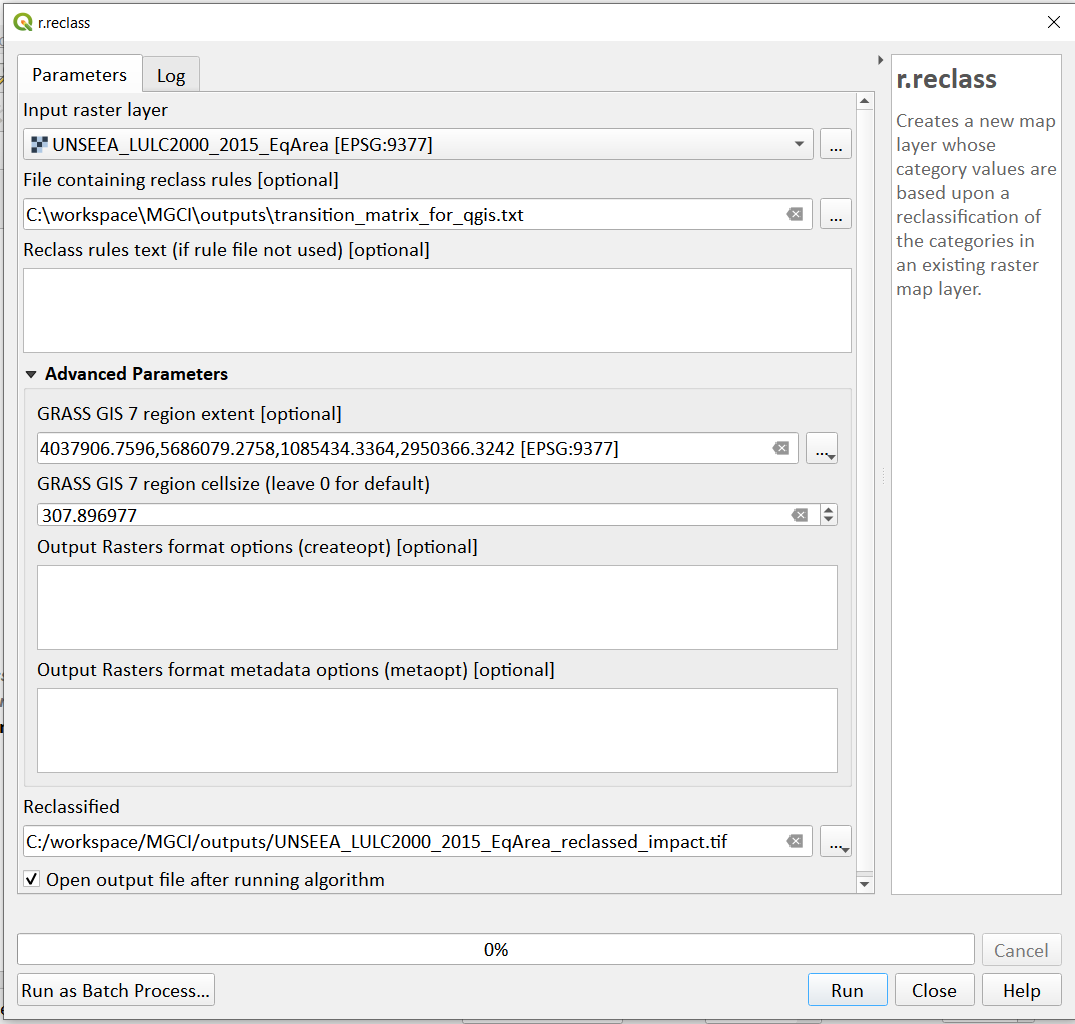
• Click Run

  (you can the two ignore the 2 warning messages that appear in red– these do not affect the correct generation of the outputs

  “ WARNING: Concurrent mapset locking is not supported on Windows”

  “ ERROR 6: C:\workspace\MGCI\outputs\UNSEEA_LULC2000_2015_EqArea_reclassed_impact.tif, band 1: SetColorTable() only supported for Byte or UInt16 bands in TIFF format.”)

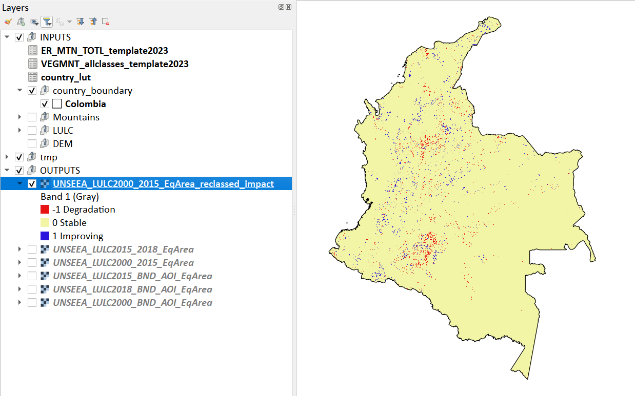
• Double-click on the output and change the symbology to paletted/unique values and click the Classify button to show the classes present in the output layer.

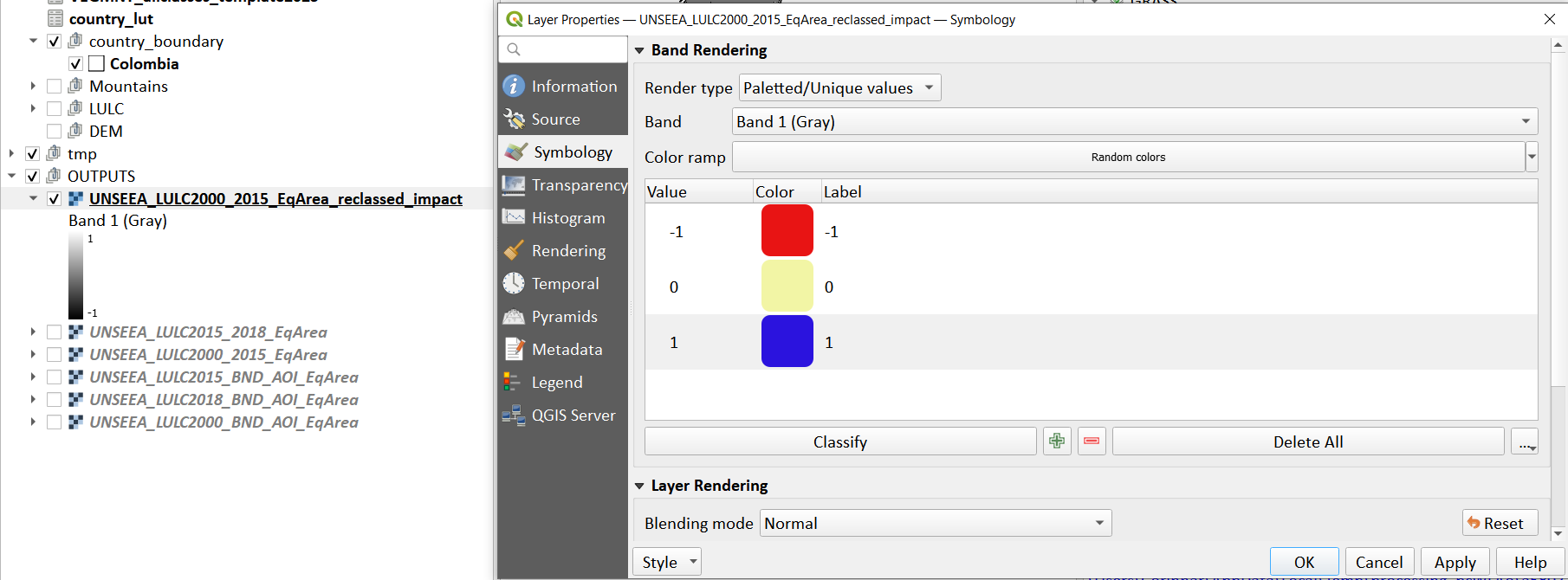
(you can also change the label to indicate 0 = stable -1 = degradation and 1 = improving)

The boundaries and names shown, and the designations used on this map do not imply official endorsement or acceptance by the United Nations.

• Repeat the above step for the next reporting period i.e. using 2015 landcover (year 1) and 2018 landcover (year2) i.e. using the layer UNSEEA_LULC2015_2018_EqArea.tif

Step-by-step equivalent of Tool B4 Combine Bioclimatic belts, LULC transitions and impact layers

The following steps are covered by this tool:

Combine landcover transitions, impact and bioclimatic belts

We now have all the layers we need for generating statistics. To make it easier we will again sum the layers together using different factors to change the values in some of the datasets.

We have the following datasets which we need to combine to generate the proportion of degraded mountain area disaggregated by LULC transitions, impact status and bioclimatic belt:

• LULC transitions (which in our case using have values 1001-10010 where LULC for year 1 has already been multiplied by 1000 and summed with year 2 values)

  **We will leave these LULC transitions dataset values as they are. **

• Bioclimatic belts (which have values 1-4 representing the 4 bioclimatic belts)

  We will multiply the bioclimatic belts by 100,000

• LULC transition impact status (values -1, 0 and 1)

  We will change the impact status by adding 2 to each of the values and multiplying by 1,000,000 thus changing values -1 to 1,000,000 (degradation) 0 to 2,000,000 (stable) and 1 to 3,000,000 (improving)

• In the processing toolbox search for the **raster calculator **

• In the expression box use the following expression (where the first dataset is the LULC transitions e.g. in this example for the baseline period, the second dataset is the Bioclimatic Belts dataset that was resampled to the resolution of the LULC dataset in the processing for sub-indicator a and the third dataset is the impact status):

  “UNSEEA_LULC2000_2015_EqArea@1” + (“MNTBelts_BND_AOI_ResampledNN_EqArea@1” *100000) + ((“UNSEEA_LULC2000_2015_EqArea_reclassed_impact@1” +2)*1000000)

  

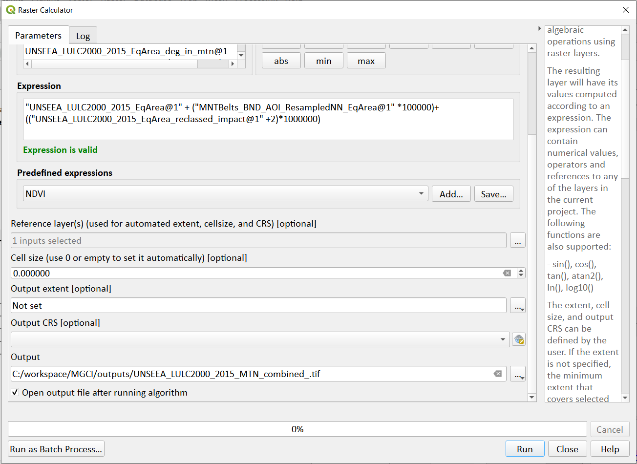
• Set the reference dataset as the UNSEEA_LULC2000_2015_EqArea@1 which is a quick way to determine the output extent, cellsize and projection of the output dataset.

• Set the output dataset as e.g. UNSEEA_LULC2000_2015_MTN_combined_.tif

• 

  The boundaries and names shown, and the designations used on this map do not imply official endorsement or acceptance by the United Nations.

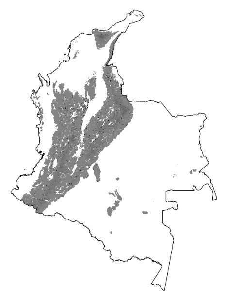
Click Run. The output is added to the table of

contents and the annotated legend below illustrates the meanings of the values

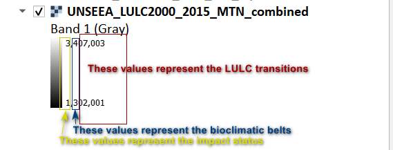
• Repeat the above step for the next reporting period i.e. using 2015 landcover (year 1) and 2018 landcover (year2)

Step-by-step equivalent of Tool B5 Generate planimetric and real surface area statistics

The following steps are covered by this tool:

NOTE: the step by step instructions only calculate planimetric area. For real Surface Area statistics the toolbox must be used.

Computation of Proportion of degraded mountain area

Generate area statistics for each land cover transition

The data are now combined and in format we can use to generate the statistics required for the sub-indicator 15.4.2b reporting. The Raster layer unique values report tool will automatically calculate planimetric area in the output and contain all the disaggregation’s we require.

This output is the main statistics table from the analysis, from which other summary statistics tables will be generated.

• In the processing toolbox search for Raster layer unique values report

• Double click on the Raster layer unique values report.

• Set the input layer to the combined layer created in the previous step

  e.g. UNSEEA_LULC2000_2015_MTN_combined_.tif.

• Under the Unique values table click on … and choose Save to File…. Enter a name for the file, in this case subIndicator_b_Areas_COL_basline2000_2015.gpkg.

  

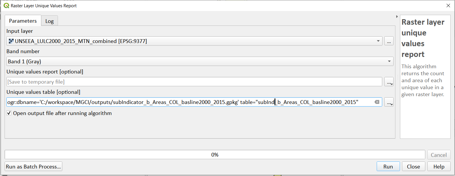
• Click Run.

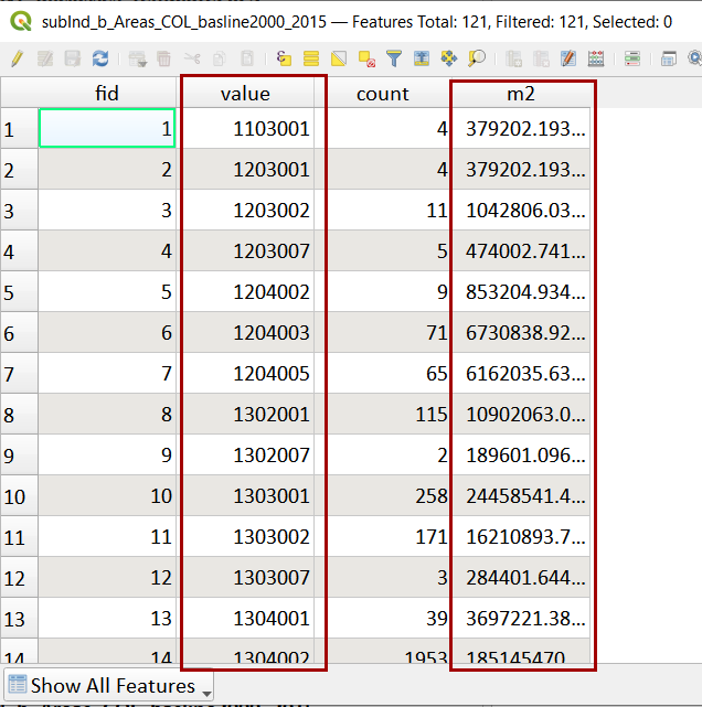
Now the subIndicator_b_Areas_COL_basline2000_2015 layer will be added to the Layers panel. Right-click on the layer and click  Open Attribute Table. The column m2 contains the area for each class in square meters.

Let’s convert the area to square kilometers. In the Processing Toolbox, search and select Vector table >> Field Calculator.

• In the Field Calculator dialog, select the subIndicator_b_Areas_COL_basline2000_2015 layer

• Enter the Field name as Area_sqkm.

• In the Result field type choose **Float  **

• In the Expression window, enter the below expression. This will convert the sqmt to sqkm and round the result to 2 decimal places. Under the Calculated click on … and choose Save To File… . Enter the name as subIndicator_b_Areas_COL_basline2000_2015_sqkm

  round(“m2”/1e6, 2)

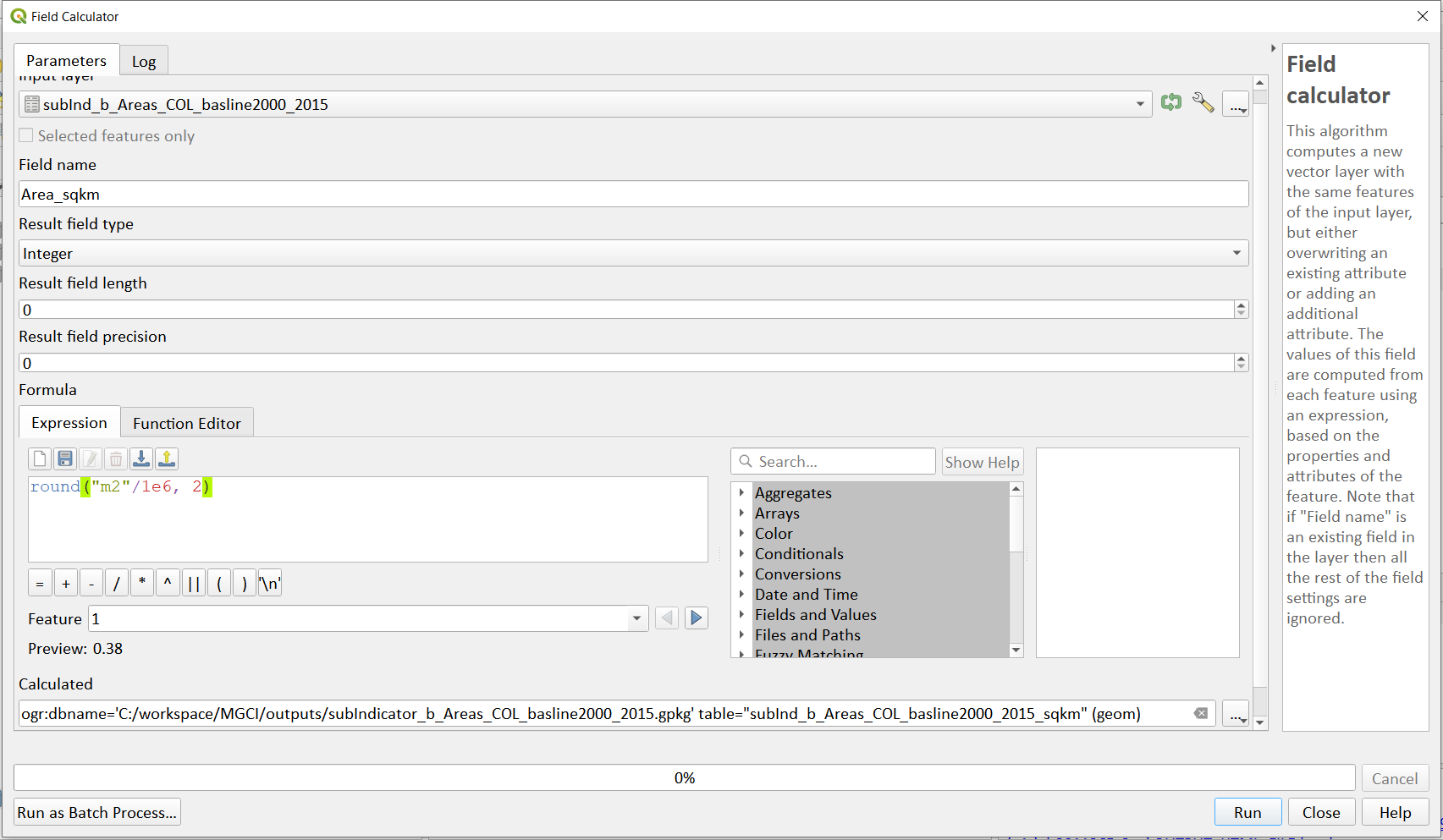
• Click Run.

Now the subIndicator_b_Areas_COL_basline2000_2015_sqkm will be loaded in canvas. Open the Attribute table and examine the newly added area_sqkm column.

As indicated before the Value column contains numbers for each unique class combination. To make the results easier to interpret. Let’s also re-add all the descriptive attributes

In the Attribute Table, click the “ Open Field Calculator” button in the top bar.

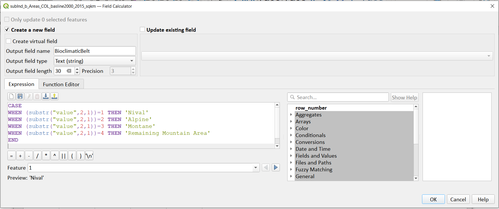
• Enter the Field name as BioclimaticBelt.

• In the Result field type, choose Text (string). In Output field length enter 100.

• In the Expression window enter the below expression. This expression uses the CASE statement to assign a value based on multiple conditions. In this case it extracts the second string of the value field, which indicate the type of land cover, to assign the name of the land cover in the new field name called “ BioclimaticBelt”

  CASE

  WHEN (substr(“value”,2,1))=1 THEN ‘Nival’

WHEN (substr(“value”,2,1))=2 THEN ‘Alpine’

WHEN (substr(“value”,2,1))=3 THEN ‘Montane’

WHEN (substr(“value”,2,1))=4 THEN ‘Remaining Mountain Area’

END

• Click on the Save button on the attribute menu to save the edits.

In the Attribute Table, click the “ Open Field Calculator” button in the top bar again.

• Enter the Field name as LULC_transition.

• In the Result field type, choose Whole Number (Integer)..

• In the Expression window enter the expression: substr(“value”,3,5)

  

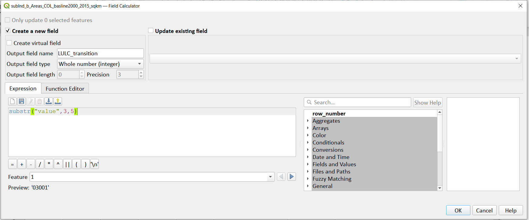
• Click OK

• Click on the Save button on the attribute menu to save the edits.

• Click on the toggle editing button to turn off the attribute editing

We can now use the LULC_transitions field to join on the rest of the attributes from the transitions matrix file.

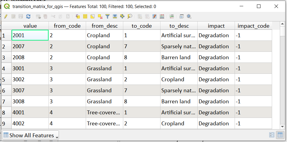
• Open the transitions_matrix_for_QGIS.csv file . It should be the one containing the following fields. We are going to use the Value field in this file to join to the LULC_transition field in our statistic file (subIndicator_b_Areas_COL_basline2000_2015_sqkm)

• Right click and select properties on the statistics file

  i.e. subIndicator_b_Areas_COL_basline2000_2015_sqkm

• Click on the joins tab and click on the green + button

• For the join layer pick the transitions matrix that you opened above

• For the join field pick Value

• For the target field pick LULC_transition

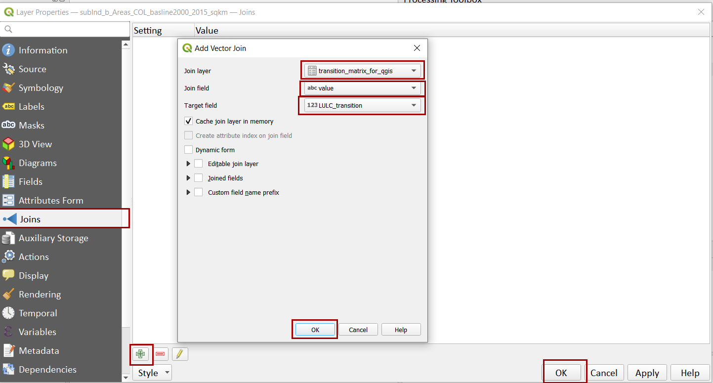
• Click OK then OK again

• You should see that a join has been added in the top panel

  

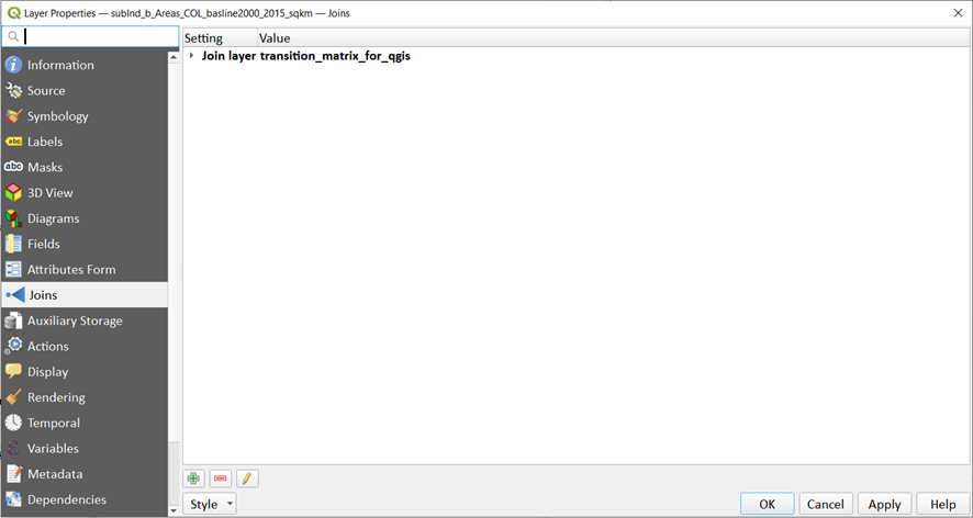
• Click OK to close the join window

• Open the attribute table of the statistics file again and you should now see that it includes the joined fields. (i.e. the subIndicator_b_Areas_COL_basline2000_2015_sqkm file )

  

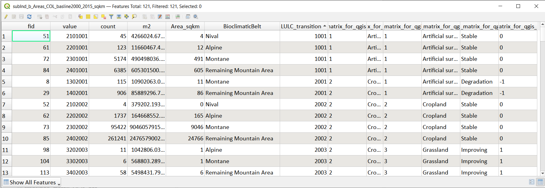
• These are only temporarily joined so we need to save as a new file. We will use the refactor field tool as this allows us to remove the joinfield preface (in this example transition_matrix_for_qgis_)that was added to the joined on fields and also set the correct output types for the other fields (as below)

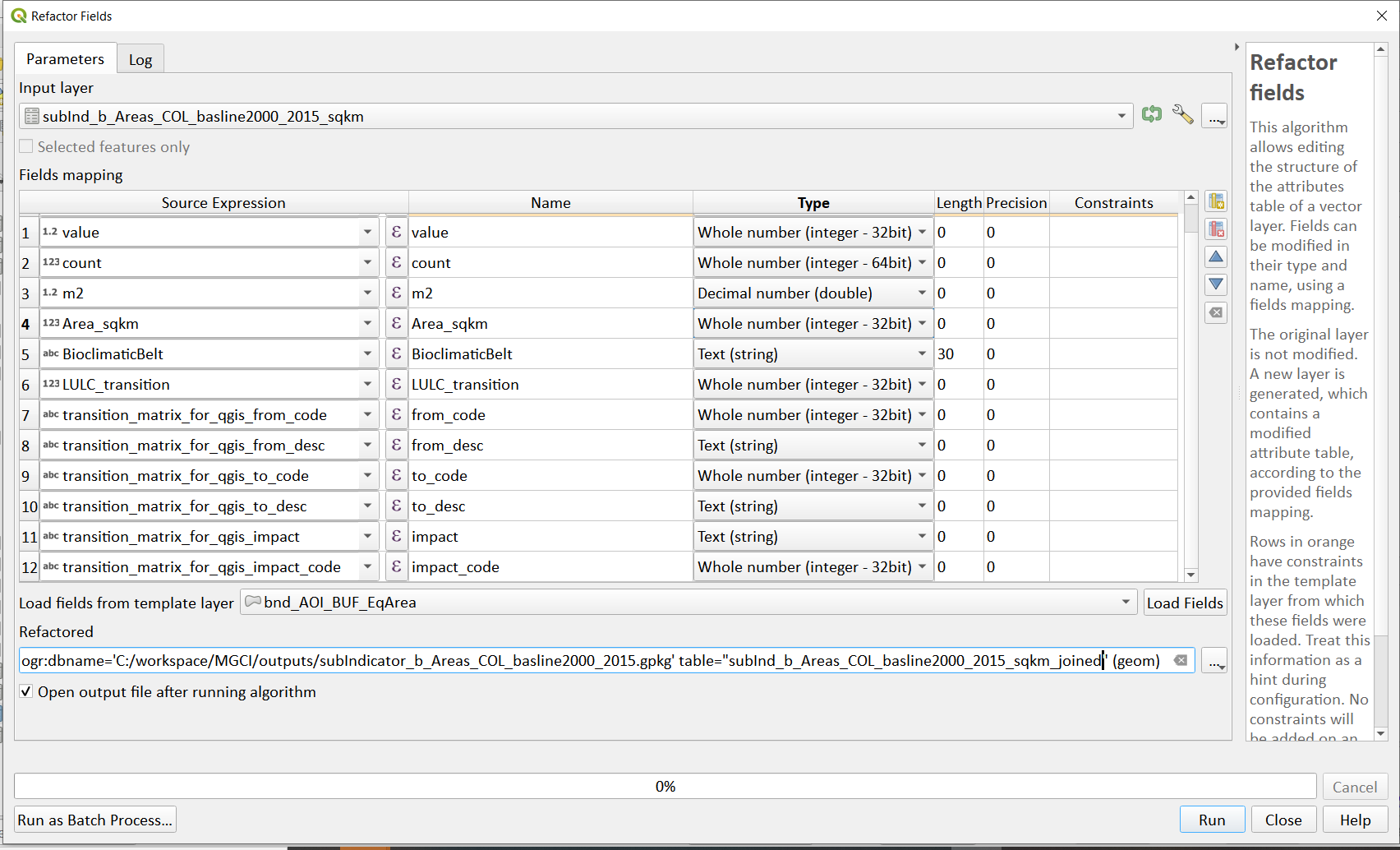
• Save the refactored file to a new name within the geopackage

  e.g. subInd_b_Areas_COL_basline2000_2015_sqkm_joined

Step-by-step equivalent of Tool B6 B6 Formatting to reporting tables

The following steps are covered by this tool:

Calculate area statistics and format statistics to reporting format

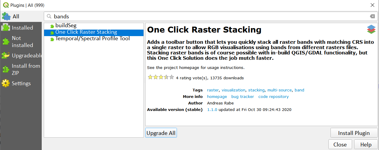
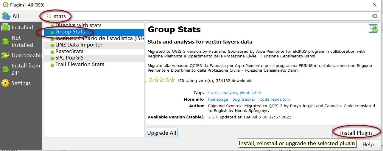
• From the main menu click on Plugins>>Manage and install plugins

• Search for stats and click on Group Stats then click on Install Plugin

• From the main menu bar click on Vector>> Groupstats >> Group stats

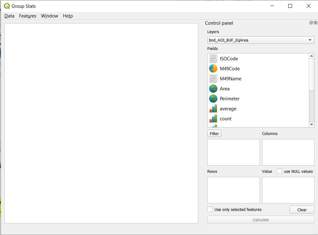
• Drag the Area_sqkm field into the Value box

• Drag sum into the Value box

• Drag BioclimaticBelt, and to_desc into the Rows box

• Drag impact into the Columns box

• Click Calculate

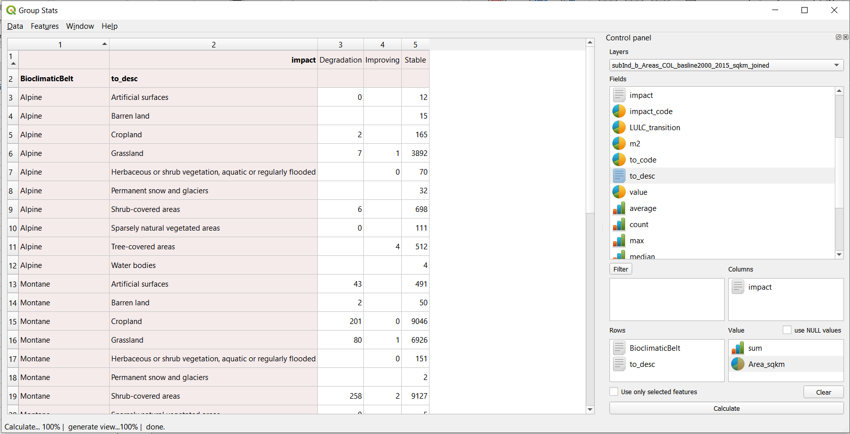
A summary table will appear in the Group Stats window

• From the Group stats menu click Data>>copy all to clipboard

• Next open Microsoft Excel with a new blank worksheet

• Paste the copied clipboard contents into the excel worksheet

  

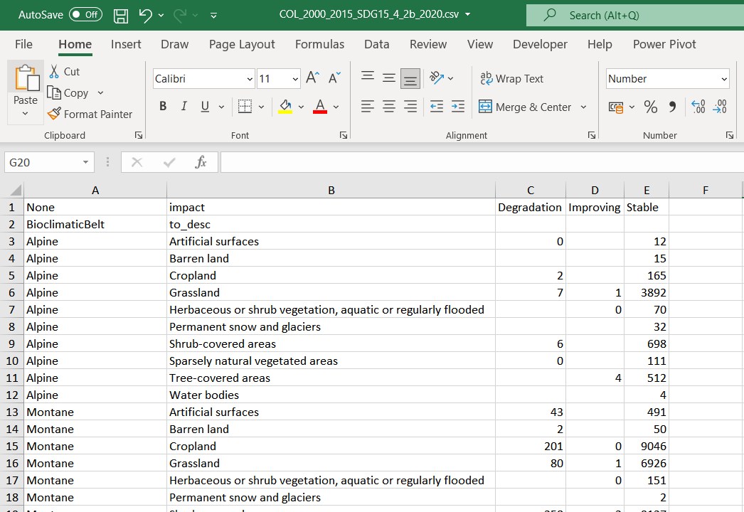
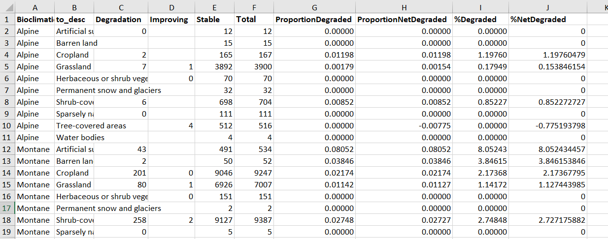
• Highlight the headings Degradation, Improving and Stable and shift them down one cell

• Highlight the entire first row and delete (with the heading None and impact)

• Add 3 new columns at the end called Total, ProportionDegraded, ProportionNetDegraded, %Degraded and %NetDegraded.

  

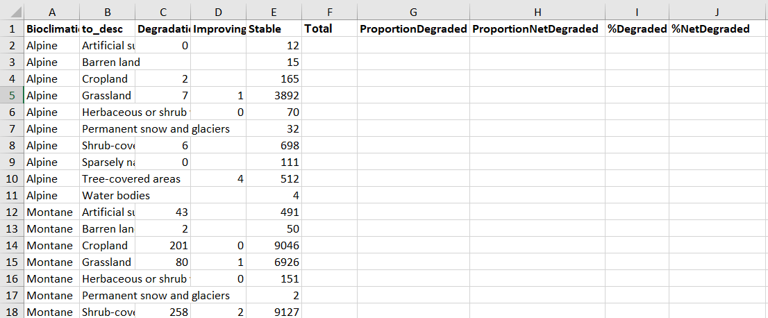
• Calculate Total to be the sum of columns C to E

• Calculate ProportionDegraded to be column C dived by column F

• Calculate ProportionNetDegraded to be column C minus column D and diving it by column F

• Calculate %Degraded and %Net Degraded to be column G and H multiplied by 100, respectively.

  

• Next insert pivot table and summarise by Bioclimatic Belt to sum the Degradation values, Improving values and Total Mountain Area

  

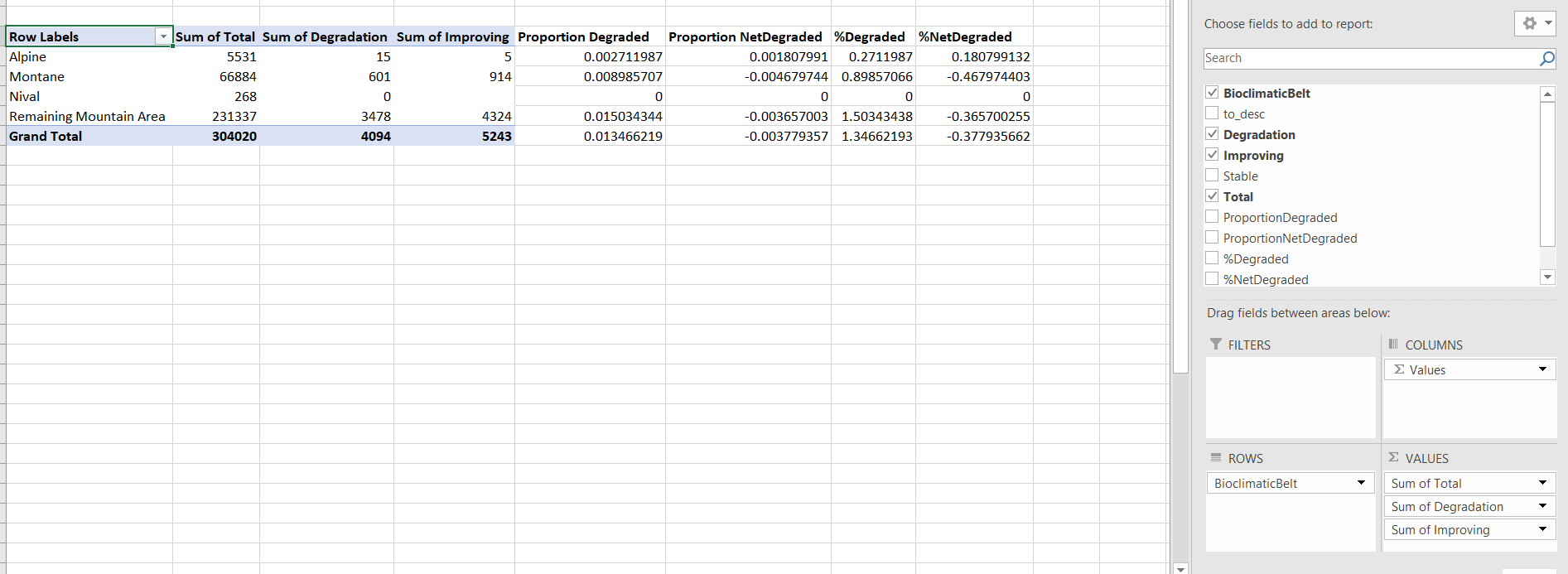
• Again add and calculate columns for ProportionDegraded, ProportionNetDegraded, %Degraded and %NetDegraded

• Save to .xlsx format e.g. COL_2000_2015_SDG15_4_2b.xls

• Repeat the above step for the next reporting period i.e. using 2015 landcover (year 1) and 2018 landcover (year2) and any other reporting periods.

END

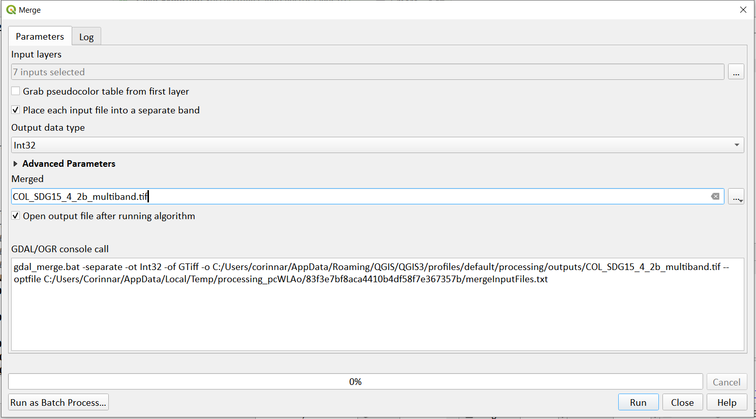
Generate multiband raster to help with spatial interrogation of results and QA

Use the gdal merge tool to combine all the input rasters into a single multi-band raster

https://gis.stackexchange.com/questions/62005/how-to-rename-the-band-names-of-a-layer-stack

https://issues.qgis.org/issues/17128

Looking at this plugin:

[1]

At the time of writing the Long Term Release of QGIS is Version 3.22 ‘Białowieża’

[2]

IPBES defines land degradation as “the many human-caused processes that drive the decline or loss in biodiversity, ecosystem functions or ecosystem services in any terrestrial and associated aquatic ecosystems” (IPBES, 2018)